近似贝叶斯计算简明教程（节选）

【摘要】似然是贝叶斯统计推断的基本要素之一，传统方法会通过对似然的参数化建模，来得到其参数的后验分布并进而得到后验预测分布。但在很多时候，似然的建模并不那么明确，甚至无法被参数化建模，使得贝叶斯分析方法陷入困难。近似贝叶斯计算（Approximate Bayesian Computation, ABC）正是解决此问题的基本方法，在最近 20 年左右时间里得到了快速发展。本文解释了一些近似贝叶斯计算的基本概念、原理和示例，帮助初学者快速掌握该方法。本书节选自 Martin 的《Bayesian modeling and computation in python》一书第八章。

【原文】 Martin, O.A., Kumar, R. and Lao, J. (2021) Bayesian modeling and computation in python. Boca Raton. https://github.com/BayesianModelingandComputationInPython/BookCode_Edition1/

在本章中，我们讨论 近似贝叶斯计算（ Approximate Bayesian Computation ， ABC ）。近似贝叶斯计算中的 “近似” 指缺乏显式的似然函数（注意：不同于后验分布的近似推断），因此近似贝叶斯计算方法的另一个常见并且更明确的名称是 无似然方法。尽管有很多学者认为这两个术语之间存在区别，不能作为可以互换的概念，但无似然方法这个名称还是更容易让初识的人理解。

当没有明确似然表达式时，近似贝叶斯计算方法会非常有用，但需要有一个能够生成合成数据的参数化 模拟器。这个模拟器有一个或多个未知参数，我们想知道哪一组参数生成的合成数据 足够接近 观测数据，然后再计算这组参数的后验分布。

近似贝叶斯计算方法在生物科学中变得越来越普遍，特别是在系统生物学、流行病学、生态学和群体遗传学等子领域^[82]。但其也可用于其他领域，因为近似贝叶斯计算能够提供一种解决许多实际问题的灵活方式。

应用的多样性也反映在近似贝叶斯计算的 Python 软件包中 ^[83]^[84]^[85] 。不过，额外的近似层也带来了一系列困难，主要是：在缺乏似然的情况下，足够接近到底指什么？如何能够实际计算一个近似的后验？

我们将在本章中从一般性角度讨论这些挑战。强烈建议有兴趣将近似贝叶斯计算方法应用于自身问题的读者，用自己领域知识中的例子来补充本章内容。

1 超越似然

根据贝叶斯定理，计算后验需要两个基本成分：先验和似然。但对于某些特定问题，可能无法以封闭形式表达似然，或者计算似然的成本过高。这对于贝叶斯热爱者来说，似乎进入了一条死胡同。

但如果能够以某种方式生成合成数据，情况可能就会有所不同。特别是当此类合成数据能够与真实观测数据足够相似时，似乎能够用该数据的生成过程来近似真实数据的似然。这种合成数据生成器通常被称为 模拟器。从近似贝叶斯计算方法角度来看，模拟器就是一个黑盒子，我们在一侧输入参数值，并从另一侧获取模拟数据。

这里的复杂性在于：不确定哪些输入参数能够生成足以与观测数据相似的合成数据。

所有近似贝叶斯计算方法共有的基本概念是：用能够计算某种距离的 $\delta$ 函数替换似然函数，或者更一般地说，计算观测数据 $Y$ 与模拟器生成数据 $\hat Y$ 之间的某种差异。

\hat Y \sim \operatorname{Sim}(\theta)

p(\theta \mid Y) \stackrel{\propto } \sim \delta(Y, \hat Y \mid \epsilon)\; p(\boldsymbol{\theta})

我们的目标是使用函数 $\delta$ 来近似似然函数：

\lim_{\epsilon \to 0} \delta(Y, \hat Y \mid \epsilon) = p(Y \mid \boldsymbol{\theta})

我们需要引入了一个容差参数 $\epsilon$ ，因为对于大多数问题，生成与观测数据 $Y$ 相等的合成数据集 $\hat Y$ 几乎不可能。 $\epsilon$ 值越大，我们对 $Y$ 和 $\hat Y$ 之间的近似程度就越能容忍。一般来说，对于给定问题，较大的 $\epsilon$ 值意味着对后验更粗略的近似。

在实践中，随着数据样本量或维度的增加，找到足够小的 $\delta$ 值将越来越困难。一个简单的解决方案是增加 $\epsilon$ 的值，但这意味着增加了近似误差。因此，更好的解决方案可能是计算一个或多个统计量 $S$ 之间的距离，而不是直接计算合成数据集和真实数据集之间的距离。

\delta\left(S(Y), S(\hat Y) \mid \epsilon\right)

当然，使用统计量会给近似贝叶斯计算带来额外的误差源，除非该统计量对于模型参数 $\theta$ 来说是充分统计量。不幸的是，并非所有情况都能满足这种要求。尽管如此，不充分统计量在实践中仍然非常有用。

在本章中，我们将探讨一些不同的距离和统计量，重点关注经过验证的一些方法。

充分统计量

如果除了某个统计量之外，从同一样本计算的其他统计量无法提供有关该样本的更多信息，则该统计量对于模型参数而言是充分的，被称为充分统计量。换句话说，该统计量足以总结你的样本而不会丢失信息。

例如，给定来自具有期望值 $\mu$ 和已知有限方差的高斯分布的独立同分布样本，样本的均值对于参数 $\mu$ 来说是一个 充分统计量。请注意，均值无法说明离散度，因此其仅对参数 $\mu$ 是充分的。

众所周知，对于独立同分布数据，具有充分统计量且维度与 $\theta$ 相同的唯一分布来自于 指数族分布 ^[86]^[87]^[88]^[89] 。对于其他类型的分布，充分统计量的维度会随着样本量的增加而增加。

2 近似的后验

执行 ABC 计算的大多数基础方法是按照一定概率做拒绝采样。我们将用 图1 以及对算法的抽象描述来逐步解释，如下所示。

（1）从先验分布中抽取 $\theta$ 的值作为提议。

（2）将该值传递给模拟器并生成合成数据。

（3）如果合成数据的距离 $\delta$ 较阈值 $\epsilon$ 更近，则保存提议的 $\theta$ ，否则拒绝它。

（4）重复直到获得所需数量的样本。

figures/ABC_rejection.png

图1：近似贝叶斯计算拒绝采样器的一个步骤。从先验分布（顶部）中抽取一组 $\theta$ 值。将每个值都被传递给模拟器，模拟器生成合成数据集（虚线分布），然后比较合成数据与观测数据（底部）的分布。在这个例子中，只有 $\theta_1$ 能够生成一个与观测数据足够接近的合成数据集，因此 $\theta_0$ 和 $\theta_2$ 被拒绝。请注意，如果仅使用统计量，则需要在第 $2$ 步之后和第 $3$ 步之前计算合成数据和观测数据的统计量信息。

ABC 拒绝采样器的主要缺点是：如果先验分布与后验分布相差太大，我们会花费大部分时间提出将被拒绝的值。因此，更好的办法是从接近真实后验的分布中提出建议值。但通常来说，我们对后验的了解不够，无法手动执行此操作，但可以使用 序贯蒙特卡洛 (SMC) 方法来实现。

序贯蒙特卡洛是一种通用采样方法，就像 MCMC 方法一样。但序贯蒙特卡洛也适用于执行近似贝叶斯计算，并被称为 “序贯蒙特卡洛-近似贝叶斯计算（ SMC-ABC ）” 。如果你想了解更多关于序贯蒙特卡洛方法的细节，可以参阅相关资料，但要理解本章，暂时只需要知道序贯蒙特卡洛是通过在 $s$ 个连续阶段中逐步增加辅助参数 $\beta$ 的值 $\{\beta_0=0 < \beta_1 < ... < \beta_s=1\}$ 实现的。其作法是：从先验（ $\beta = 0$ ）开始采样，直到到达后验（ $\beta = 1$ ）。因此，可以将 $\beta$ 视为一个逐渐开启似然的参数。 $\beta$ 的中间值序列由序贯蒙特卡洛方法自动计算。数据相对于先验的信息越多和（/或）后验几何形态越复杂，则序贯蒙特卡洛所采取的中间步骤就会越多。

图 2 显示了一个假设的中间分布序列，从浅灰色的先验到蓝色的后验。

figures/smc_tempering.png

图2：序贯蒙特卡洛采样器探索的退火后验序列，从浅灰色的先验 ( $\beta = 0$ ) 到蓝色的真实后验 ( $\beta = 1$ )。开始时较低的 $\beta$ 值有助于防止采样器卡在单一最值中。

3 用近似贝叶斯计算拟合一个高斯

让我们用一个简单的例子先热热身，从均值为 $0$ 、标准差为 $1$ 的高斯分布数据中估计均值和标准差。对于这个问题，我们可以拟合模型：

\begin{split} \boldsymbol{\mu} \sim &\; \mathcal{N}(0, 1) \\ \boldsymbol{\sigma} \sim &\; \mathcal{HN}(1) \\ \boldsymbol{s} \sim &\; \mathcal{N}(\boldsymbol{\mu}, \boldsymbol{\sigma}) \end{split}

在 PYMC3 中编写此模型的方法见代码 gauss_abc:

with pm.Model() as gauss:     
  μ = pm.Normal("μ", mu=0, sigma=1)     
  σ = pm.HalfNormal("σ", sigma=1)     
  s = pm.Normal("s", μ, σ, observed=data)     
  trace_g = pm.sample()

使用 SMC-ABC 的等效模型见代码:

with pm.Model() as gauss:     
  μ = pm.Normal("μ", mu=0, sigma=1)     
  σ = pm.HalfNormal("σ", sigma=1)     
  s = pm.Simulator("s", normal_simulator, params=[μ, σ],
                   distance="gaussian", sum_stat="sort",
                   epsilon=1, observed=data)
  trace_g = pm.sample_smc(kernel="ABC")

可以看到两种代码之间有两个重要的区别：

使用了 pm.Simulator 分布
使用 pm.sample_smc(kernel="ABC") 代替了 pm.sample()。

通过使用 pm.Simulator ，我们告诉 PyMC3，不会对似然使用封闭形式表达式，而是定义一个伪似然。此时需要传递一个生成合成数据的 Python 函数，本例中该函数为 normal_simulator 以及其参数 params=[μ, σ] 。模拟器代码给出了 normal_simulator 函数的定义，样本大小为 $1000$ ，未知参数为 $\mu$ 和 $\sigma$ :

1
2
3


def normal_simulator(μ, σ):
    return np.random.normal(μ, σ, 1000)

我们还需要向 pm.Simulator 传递其他可选参数，包括距离函数 distance、统计量信息 sum_stat 和阈值 epsilon 的值。此外，还要将观测数据以常规似然形式传递给 pm.Simulator 。

通过使用 pm.sample_smc(kernel="ABC") ，我们告诉 PYMC3 在模型中寻找 pm.Simulator 并使用它来定义伪似然，其余的采样过程与序贯蒙特卡洛算法中描述的相同。当 pm.Simulator 存在时，其他采样器将无法运行。

本例中的 normal_simulator 函数原则上可以是任何我们想要的 Python 函数，实际上甚至可以是经过封装的非 Python 代码，例如 Fortran 或 C 代码。这就是近似贝叶斯计算方法的灵活性所在。在本例中，模拟器只是一个 NumPy 随机生成器函数的包装器。

与其他采样器一样，建议运行多个链，以便诊断采样器是否无法正常工作，PyMC3 将尝试自动执行此操作。 图 3 显示了使用两条链运行代码 gauss_abc 的结果。

可以看到，我们能够恢复真实参数，并且采样器没有出现任何明显的采样问题。

figures/trace_g.png

图 3: 正如预期的 $\mu \approx 0$ 和 $\sigma \approx 1$ 一样，两条链都支持核密度估计和秩图反映的后验。请注意，这两条链中都是通过运行 $2000$ 个并行 SMC 链获得的，如 SMC 算法中所述。

4 选择距离函数、阈值和统计量

如何定义有效的距离度量、统计量和阈值 $\epsilon$ 取决于待解决的问题。这意味着我们应该在获得结果之前进行一些试验和尝试，尤其是在遇到新问题时。像往常一样，事先对方案做充分思考有助于减少备选的数量；不过我们也应该习惯于运行实验，因为它总是有助于更好地理解问题，并对超参数做出更明智的抉择。

在接下来的部分中，我们将讨论一些比较通用的指南。

4.1 距离函数的选择

上例中，我们使用了默认距离函数 distance="gaussian" 来运行代码 gauss_abc，其定义为：

\sum_i - \frac{||X_{oi} - X_{si}||^2}{2 \epsilon_i^2} \tag{6}

其中 $X_{o}$ 是观测数据， $X_{s}$ 是模拟数据， $\epsilon$ 是其缩放参数。我们称 图 6 为高斯的，因为它在对数尺度上是高斯核。我们使用对数尺度来计算伪似然，就和在实际似然（和先验）中一样。 $||X_{oi} - X_{si}||^2$ 是欧几里得距离（也称为 $L2$ 范数），因此也可以将公式 图 6 描述为加权欧几里得距离。这是目前比较流行的选择，其他选项还有：在 PYMC3 中被称为拉普拉斯距离的 $L1$ 范数（绝对差的和）； $L-\infty$ 范数（差的最大绝对值）；马氏距离： $\sqrt{(xo - xs )^{T}\Sigma(xo - xs)}$ ， $\Sigma$ 为协方差矩阵。

高斯距离、拉普拉斯等可以应用于整个数据，或者应用于统计量。此外，还专门引入了一些能够避免统计量计算、但效果也很好的距离函数 ^[90]^[91]^[92]。我们将介绍其中的 Wasserstein 距离 和 KL 散度。

在代码 gauss_abc 中，我们使用了 sum_stat="sort" ，这告诉 PYMC3 在计算公式 图 6 之前对数据进行排序。这相当于计算 一维 2-Wasserstein 距离，如果使用 $L1$ 范数，则将得到 一维 1-Wasserstein 距离。当然，也可以为大于 $1$ 的维度定义 Wasserstein 距离（ ^[92] ）。

在计算距离之前对数据排序，会使分布之间的比较更加公平。想象一下，如果有两个完全相等的样本，但是一个从低到高排序，另一个是高到低排序。此时应用公式 图 6 这样的度量，会得出“两个样本不同”的结论。但如果先排序而后计算距离，会得出“两个样本相同”结论。这是一个非常极端的场景，但有助于阐明数据排序背后的直觉。此外，对数据进行排序的前提，是假设我们只关心数据分布，不关心数据顺序；否则的话，做排序处理会破坏数据中本来存在的结构。

为了避免定义和计算统计量而引入的另一个距离是使用 KL 散度（参见第 {ref}DKL 部分）。通常使用以下表达式来近似计算 KL 散度（ ^[90]^[91] ）：

\frac{d}{n} \sum \left(- \frac{\log(\frac{\nu_d}{\rho_d})}{\epsilon} \right) + \log\left(\frac{n}{n-1}\right)

其中 $d$ 是数据集的维度（变量或特征的数量）， $n$ 是观测数据点的数量。 $\nu_d$ 包含观测数据到模拟数据的 1-最近邻距离， $\rho_d$ 包含观测数据到自身的 2-最近邻距离（注意，如果你将数据集与其自身进行比较，则 1-最近邻距离 永远为零）。由于该方法涉及最近邻搜索的 $2n$ 次操作，因此通常使用 k-d 树 来实现 ^[93] 。

4.2 阈值的选择

在许多近似贝叶斯计算方法中， $\epsilon$ 参数用作硬阈值，生成距离大于 $\epsilon$ 的样本的参数 $\theta$ 值将被拒绝。此外， $\epsilon$ 可以是用户必须设置的递减值列表，或者算法自适应找到的结果。

在 PYMC3 中， $\epsilon$ 采用的是距离函数的尺度，就像在公式 图 6 中一样，所以不能用作硬阈值。我们可以根据需要设置 $\epsilon$ 。我们可以选择一个标量值（相当于将所有 $i$ 的 $\epsilon_i$ 设置为相等）。这在评估数据上的距离而不是统计量上的距离时非常有用。在此情况下，合理猜测可能是数据的经验标准差。

如果我们改为使用统计量，那么可以将 $\epsilon$ 设置为值列表。这通常是必要的，因为每个统计量可能具有不同的尺度。如果尺度差异太大，那么每个统计量的贡献将是不均衡的，甚至可能出现单个统计量主导距离计算的情况。在此情况下， $\epsilon$ 的一个常用选择是在先验预测分布下的 $i^{\text{th}}$ 个统计量的经验标准差，或中值绝对差，因为这样选择相对于异常值来说更为稳健。使用先验预测分布的问题之一是其可能比后验预测分布更宽，因此，为了找到一个合适的 $\epsilon$ 值，我们可能希望将上述有依据的猜测作为上限，然后从这些值中尝试一些较低的值。然后我们可以根据计算成本、所需的精度/误差水平和采样器的效率等几个因素来选择 $\epsilon$ 的最终值。一般来说， $\epsilon$ 的值越低，近似值就越好。

图 4 显示了 $\mu$ 和 $\sigma$ 的几个 $\epsilon$ 阈值设置以及 NUTS 采样的森林图（使用正常似然而不是模拟器）。

figures/trace_g_many_eps.png

图 4: $\mu$ 和 $\sigma$ 的森林图，使用 NUTS 或近似贝叶斯计算获得， $\epsilon$ 为 $1$ 、 $5$ 和 $10$ 的递增值。

减小 $\epsilon$ 的值并非毫无限制的，因为过低的值有时会使采样器非常低效，表明目标是一个没有太大意义的准确度水平。图 5 显示了当来自代码 gauss_abc 的模型以 epsilon=0.1 的值进行采样时，序贯蒙特卡洛采样器难以收敛，采样器非常失败。

figures/trace_g_eps_too_low.png

图 5: 模型trace_g_001的核密度估计和秩图，收敛失败表明 $\epsilon=0.1$ 的取值对于该问题来说太苛刻了。

为了能够为 $\epsilon$ 确定一个好的值，可以使用一些非近似贝叶斯计算方法中的模型评价工具，例如贝叶斯 $p$ 值和后验预测检查，如图 图 6、图 7 和 图 8。 图 6 包含值 $\epsilon=0.1$ ，主要是为了展示校准不佳的模型。但在实践中，如果获得像 图 5 中的秩图，我们应该停止分析计算得到的后验，并重新检查模型定义。此外，对于近似贝叶斯计算方法，还应检查超参数 $\epsilon$ 的值、统计量或距离函数。

figures/bpv_g_many_eps_00.png

图 6： $\epsilon$ 值递增的边缘贝叶斯 $p$ 值分布。对于一个校准良好的模型，我们应该预期一个均匀分布。可以看到 $\epsilon=0.1$ 的校准很糟糕，因为 $\epsilon$ 的值也是如此。对于 $\epsilon$ 的所有其他值，分布看起来更加均匀，并且均匀性水平随着 $\epsilon$ 的增加而降低。se 值是预期均匀分布和核密度估计之间的（缩放的）平方差。

figures/bpv_g_many_eps_01.png

图 7：增加 $\epsilon$ 值的贝叶斯 $p$ 值。蓝色曲线是观测分布，灰色曲线是预期分布。对于一个校准良好的模型，我们期望分布集中在 $0.5$ 左右。可以看到 $\epsilon=0.1$ 的校准很糟糕，因为 $\epsilon$ 的值太低了。可以看到 $\epsilon=1$ 提供了最好的结果。

figures/ppc_g_many_eps.png

图 8： $\epsilon$ 递增时的后验预测检查。蓝色曲线是观测分布，灰色曲线是预期分布。令人惊讶的是，从 $\epsilon=0.1$ 中似乎得到了一个很好的调整，即便我们知道来自该后验的样本不可信。这是一个非常简单的例子，我们完全靠运气得到了正确答案。这是一个 a too good to be true fit 的例子。实际上这是最糟糕的！如果我们只考虑具有看起来合理的后验样本的模型（即不是 $\epsilon=0.1$ ），则可以看到 $\epsilon=1$ 提供了最好的结果。

4.3 统计量的选择

统计量的选择可能比距离函数的选择更难，并且会产生更大的影响。

出于此原因，许多研究都集中在这个主题上，从使用不需要统计量的距离 ^[91]^[92] 到选择统计量的策略 ^[94]。

一个好的统计量提供了低维度和信息量之间的平衡。当我们没有足够统计量数据时，很容易通过添加大量统计量数据来进行过度补偿。直觉是信息越多越好。然而，增加统计量的数量实际上会降低近似后验 ^[94] 的质量。对此的一种解释是，我们从计算数据上的距离转移到计算摘要上的距离以减少维度，通过增加我们正在违背该目的的摘要统计数据的数量。

在一些领域，如群体遗传学，近似贝叶斯计算方法非常普遍，人们开发了大量有用的统计量数据 ^[95]^[96]^[97]。一般来说，查看你正在研究的应用领域的文献以了解其他人在做什么是一个好主意，因为他们已经尝试并测试了许多替代方案的机会很高。

如有疑问，我们可以遵循上一节中的相同建议来评估模型拟合，即秩图、贝叶斯 $p$ 值、后验预测检查等，并在必要时尝试替代方案（参见图 图 5， 图 6、图 7 和 图 8）。

5 g-and-k 分布

一氧化碳 ( $CO$ ) 是一种无色、无味的气体，大量吸入有害甚至致命。当某物燃烧时会产生这种气体，尤其是在氧气含量低的情况下。世界上许多城市通常会监测一氧化碳和其他气体，如二氧化氮 ( $NO_2$ )，以评估空气污染程度和空气质量。在城市中，一氧化碳的主要来源是汽车以及其他燃料化石车辆或机械。 图 9 显示了 $2010$ 年至 $2018$ 年布宜诺斯艾利斯市一个站点测量的每日 $CO$ 水平的直方图。

正如我们所见，数据似乎略微向右偏。此外，数据显示了一些具有非常高的观测值。

底部子图省略了 $3$ 到 $30$ 之间的 $8$ 个观测值。

figures/co_ppm_bsas.png

图 9: $CO$ 水平的直方图。顶部子图显示整个数据，底部子图忽略了大于 $3$ 的值。

为了拟合这些数据，我们将引入单变量 g-and-k 分布。这是一个 $4$ 参数的分布，能够描述具有高偏度和/或高峰度的数据 ^[13]^[99]。g-and-k 分布的密度函数没有封闭形式的表达式，并且通过其分位数函数（即累积分布函数的逆函数）来进行定义：

a + b \ \left(1 + c \ \text{tanh}\left[\frac{gz(x)}{2}\right]\right) \left(1+z(x)^2\right)^k z(x)

其中 $z$ 是标准高斯累积分布函数的逆函数， $x \in (0,1)$ 。

（1）参数 $a$ 、 $b$ 、 $g$ 和 $k$ 分别为位置、尺度、偏度和峰度参数。如果 $g$ 和 $k$ 均为 $0$ ，则恢复了具有均值 $a$ 和标准差 $b$ 的高斯分布。

（2） $g > 0$ 给出正（右）偏度， $g < 0$ 给出负（左）偏度。参数 $k \geqslant 0$ 给出的尾部比高斯分布长，而 $k < 0$ 的尾部比高斯分布短。

（3） $a$ 和 $g$ 可以取任何实数值。通常将 $b$ 限制为正数并且 $k \geqslant -0.5$ 或有时 $k \geqslant 0$ （即尾部与高斯分布中的尾部一样重或更重）。

（4）此外，通常固定 $c=0.8$ 。

有了所有这些限制，我们可以保证得到一个严格递增的分位数函数 ^[99]，而这正是连续分布函数的标志。

代码 gk_quantile 定义了 g-and-k 分位数分布。我们省略了 cdf 和 pdf 的计算，因为涉及太多额外内容，而且在我们的例子中暂时用不到。

虽然 g-and-k 分布 的概率密度函数可以用数值方法推算 ^[99]^[100]，但使用反演方法从 g-and-k 模型 中进行模拟更直接和快捷 ^[101]^[100]。

为了实现反演方法，我们对 $x \sim \mathcal{U}(0, 1)$ 进行采样并替换公式 {eq}eq:g_and_k。代码 gk_quantile 展示了如何在 Python 中执行此操作，图 10 展示了 g-and-k 分布 的示例。

class g_and_k_quantile:
    def __init__(self):
        self.quantile_normal = stats.norm(0, 1).ppf

    def ppf(self, x, a, b, g, k):
        z = self.quantile_normal(x)
        return a + b * (1 + 0.8 * np.tanh(g*z/2)) * ((1 + z**2)**k) * z

    def rvs(self, samples, a, b, g, k):
        x = np.random.normal(0, 1, samples)
        return ppf(self, x, a, b, g, k)

figures/gk_quantile.png

图 10: 第一行显示了分位数函数，也称为累积分布函数（ CDF ）的逆函数。给定一个分位数值，它会返回代表该分位数的变量值。例如，如果你有 $P(X <= x_q) = q$ ，则将 $q$ 传递给分位数函数可以得到 $x_q$ 。图中第二行显示了（近似的）概率密度函数。对于此示例，使用核密度估计可以直接从代码 gk_quantile 生成的随机样本中计算得到概率密度函数。

要使用 SMC-ABC 拟合 g-k 分布，可以使用高斯距离和 sum_stat="sort"。或者，也可以考虑为这个问题量身定制的统计量。参数 $a$ 、 $b$ 、 $g$ 和 $k$ 分别与位置、尺度、偏度和峰度相关联。因此，可以用这些量的稳健估计来作为新的专用统计量 ^[101] ：

\begin{split} sa &= e4 \\ sb &= e6 - e2 \\ sg &= (e6 + e2 - 2*e4)/sb \\ sk &= (e7 - e5 + e3 - e1)/sb \\ \end{split}

其中 $e1$ 到 $e7$ 是八分位数，即将样本分成八个子集的分位数。

如果注意，可以看到 $sa$ 是中位数， $sb$ 是四分位数范围，它们分别作为位置和离散度的稳健估计量。 $sg$ 和 $sk$ 看起来有点模糊，但它们分别是偏度 ^[102] 和峰度 ^[103] 的稳健估计量。

对于对称分布， $e6-e4$ 和 $e2-e4$ 将具有相同的幅度但符号相反，此时 $sg$ 将为零，而对于偏斜分布， $e6-e4$ 将大于 $ e2-e4$ 或相反。

当 $e6$ 和 $e2$ 附近的概率质量减少时（即当质量从分布的中心部分移动到尾部时）， $sk$ 的分子项在增加。而 $sg$ 和 $sk$ 中的分母都充当了归一化因子。

综合分析后，可以使用 Python 为问题创建新的统计量，如以下代码所示。

def octo_summary(x):
    e1, e2, e3, e4, e5, e6, e7 = np.quantile(
        x, [.125, .25, .375, .5, .625, .75, .875])
    sa = e4
    sb = e6 - e2
    sg = (e6 + e2 - 2*e4)/sb
    sk = (e7 - e5 + e3 - e1)/sb
    return np.array([sa, sb, sg, sk])

现在我们需要定义一个模拟器，只需将之前在代码 gk_quantile 中定义的 g_and_k_quantile() 函数的 rvs 方法封装起来即可。

gk = g_and_k_quantile()

def gk_simulator(a, b, g, k):
    return gk.rvs(len(bsas_co), a, b, g, k)

在定义了统计量和模拟器并导入数据之后，就可以定义模型了。

对于这个例子，基于所有参数都限制为正的事实，可以使用弱信息先验。 $CO$ 水平不能取负值，因此 $a$ 为正值； $g$ 也预计为 $0$ 或正值，因为大部分测量值预计为“low”，只有某些测量值值较大。我们也有理由假设参数很有可能低于 $1$ 。

with pm.Model() as gkm:
    a = pm.HalfNormal("a", sigma=1)
    b = pm.HalfNormal("b", sigma=1)
    g = pm.HalfNormal("g", sigma=1)
    k = pm.HalfNormal("k", sigma=1)
    
    s = pm.Simulator("s", gk_simulator,
    params=[a, b, g, k],        
                     sum_stat=octo_summary,
                     epsilon=0.1,
                     observed=bsas_co)
    
    trace_gk = pm.sample_smc(kernel="ABC", parallel=True)

图 11 显示了拟合后 gkm 模型 的配对图。

figures/pair_gk.png

图 11：分布略微偏斜，并且具有一定程度的峰度，正如所预计的那样，少量的 $CO$ 水平比其他大部分情况要高出一到两个数量级。可以看到 $b$ 和 $k$ （略微）相关。这也是可预期的，因为随着尾部密度（峰度）的增加，离散度会同时增加，但如果 $k$ 增加，g-and-k 分布可以保持 $b$ 较小。这就像 $k$ 在吸收离散度一样，有点类似于在学生 $t$ 分布中使用的尺度和 $\nu$ 参数的情况。

6 移动平均模型的近似

移动平均 (MA) 模型是建模单变量时间序列的常用方法。 $MA(q)$ 模型指定输出变量线性依赖于随机项 $\lambda$ 的当前值和 $q$ 个历史值， $q$ 被称为 MA 模型 的阶数。

y_t = \mu + \lambda_t + \theta_1 \lambda_{t-1} + \cdots + \theta_q \lambda_{t-q}

其中 $\lambda$ 是高斯白噪声误差项。

这里将使用 ^[104] 中的玩具模型。在该例中，使用均值为 $0$ 的 $MA(2)$ 模型（即 $\mu =0$ )，模型如下所示：

y_t = \lambda_t + \theta_1 \lambda_{t-1} + \theta_2 \lambda_{t-2}

如下代码（ ma2_simulator_abc ）显示了此模型的 Python 模拟器，在 图 12 中，可以看到 $\theta1 = 0.6$ 、 $\theta2=0.2$ 时该模拟器的两个实现。

def moving_average_2(θ1, θ2, n_obs=200):
    λ = np.random.normal(0, 1, n_obs+2)
    y = λ[2:] + θ1*λ[1:-1] + θ2*λ[:-2]
    return y

figures/ma2_simulator_abc.png

图 12： $MA(2)$ 模型的两种实现， $\theta1=0.6$ ， $\theta2 =0.2$ 。左列为核密度估计，右列为时间序列。

理论上，我们可以尝试想要的任何距离函数和/或统计量来拟合 $MA(q)$ 模型，但此处我们不会这样做，而是使用 $MA(q)$ 模型的一些属性作为牵引。时间序列的自相关性是 $MA(q)$ 模型的一个重要属性。理论表明，对于 $MA(q)$ 模型，大于 $q$ 的滞后效应为零，因此对于 $MA(2)$ ，使用滞后 $1$ 和滞后 $2$ 的自相关函数作为统计量似乎也是合理的。此外，为了避免计算数据的方差，我们将使用自协方差函数而不是自相关函数。

1 2	def autocov(x, n=2): return np.array([np.mean(x[i:] * x[:-i]) for i in range(1, n+1)])

此外，除非引入一些约束，否则 $MA(q)$ 模型是不可识别的。对于 $$MA(1)$$ 模型，约束为 $-1<\theta_1<1$ 。对于 $MA(2)$ ，约束为 $-2<\theta_1<2$ 、 $\theta_1 + \theta_2 > -1$ 和 $\theta_1 - \theta_2 < 1$ ，这意味着需要从一个三角形中采样，如 图 14。

结合自定义的统计量和可识别约束的近似贝叶斯计算模型见如下代码 MA2_abc 。

with pm.Model() as m_ma2:
    θ1 = pm.Uniform("θ1", -2, 2)
    θ2 = pm.Uniform("θ2", -1, 1)
    p1 = pm.Potential("p1", pm.math.switch(θ1+θ2 > -1, 0, -np.inf))
    p2 = pm.Potential("p2", pm.math.switch(θ1-θ2 < 1, 0, -np.inf))

    y = pm.Simulator("y", moving_average_2, 
                     params=[θ1, θ2],
                     sum_stat=autocov,
                     epsilon=0.1,
                     observed=y_obs)

    trace_ma2 = pm.sample_smc(3000, kernel="ABC")

pm.Potential 是一种无需向模型添加新变量，即可将任意项合并到（伪）似然的方法。引入约束特别有用。在代码 MA2_abc 中，如果 pm.math.switch 中的第一个参数为真，则我们将 $0$ 与似然相加，否则为 $-\infty$ 。

figures/ma2_trace.png

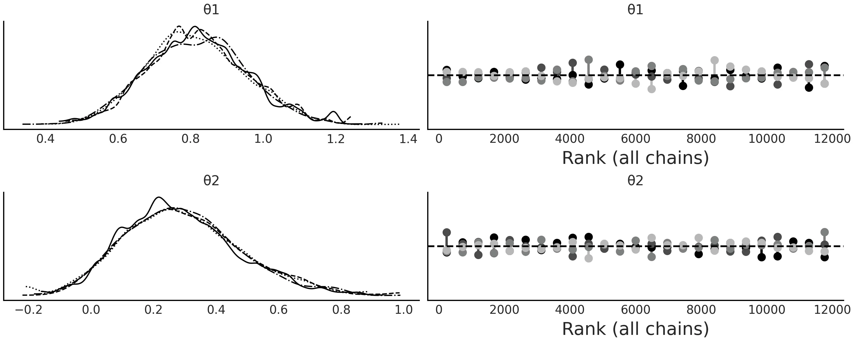
图 13: $MA(2)$ 模型的近似贝叶斯计算轨迹图。正如预计的那样，真实参数被恢复，秩图看起来非常平坦。

figures/ma2_triangle.png

图 14: 代码 MA2_abc 中定义的 $MA(2)$ 模型的近似贝叶斯计算后验。中间的子图为 $\theta1$ 和 $\theta2$ 的联合后验分布，两侧为其边缘分布；灰色的三角形代表先验分布；均值用黑色的点表示。

7 在近似贝叶斯计算的场景中做模型比较

近似贝叶斯计算方法经常用于模型选择。虽然已经提出了许多模型比较方法 ^[94]^[105]，但此处将重点讨论两种方法：贝叶斯因子法（包括与 LOO 的比较）和 随机森林法 ^[97]。

与参数推断一样，在模型比较中统计量的选择至关重要。当使用模型的预测结果来评估多个模型时，如果它们都做出了大致相同的预测，则我们无法偏爱其中任何一个模型。相同的思想可以应用于（含统计量的）近似贝叶斯计算场景下的模型比较和选择。如果使用均值作为统计量，而模型预测的均值相同，那么此统计量将不足以区分模型的优劣。

我们应该花更多时间来思考是什么让模型与众不同。

7.1 贝叶斯因子法

用于做模型比较的一个常见量是边缘似然。通常这种比较采用边缘似然比的形式，即贝叶斯因子。如果贝叶斯因子的值大于 $1$ ，则分子中的模型优于分母中的模型，反之亦然。在 {ref}Bayes_factors 中，我们讨论了有关贝叶斯因子的更多细节，包括其注意事项。其中一个警示是边缘似然通常难以计算。幸运的是，SMC 方法和扩展的 SMC-ABC 方法能够将边缘似然的计算转变成采样的副产品。 PYMC3 中的 SMC 计算并保存轨迹中的对数边缘似然，因此可以通过执行 trace.report.log_marginal_likelihood 来访问对数边缘似然的值。考虑到该值采用对数刻度，因此在计算贝叶斯因子时可以这样做：

1
2
3

ml1 = trace_1.report.log_marginal_likelihood
ml2 = trace_2.report.log_marginal_likelihood
np.exp(ml1 - ml2)

当使用统计量时，通常不能用近似贝叶斯计算方法得出的边缘似然来比较竞争中的模型 ^[106]，除非统计量对于模型比较来说是充分的。这一点非常令人沮丧，因为除了一些形式化示例或特定模型之外，没有通用的指南来确保模型的充分性 ^[106] 。如果使用所有数据（即不依赖统计量）则不存在问题。这类似于 {ref}Bayes_factors 中的讨论，即计算边缘似然通常是比计算后验困难得多的问题。即便我们设法找到了足以计算后验的统计量，也不能保证它对模型比较也有效。

为了更好地理解边缘似然在近似贝叶斯计算中的表现，现在将分析一个简短的实验。该实验中还包含 LOO，因为我们认为 LOO 是比边缘似然和贝叶斯因子更好的整体指标。

实验的基本方法是将具有显式似然的模型的对数边缘似然值、使用 LOO 计算的值、近似贝叶斯计算模型（采用含统计量和不含统计量的模拟器）的值进行比较。结果显示在图 图 14 中，和代码 gauss_nuts 以及代码 gauss_abc 中的。边缘（伪）似然值由 SMC 和 LOO 值（调用 az.loo() 函数）的乘积计算得出。请注意，LOO 是在逐点的对数似然值上定义的，而在近似贝叶斯计算中，我们只能访问逐点的对数伪似然值。

从 图 15 中可以看到，通常 LOO 和对数边缘似然的表现相似。从第一列中可以看到，model_1 始终被选为比 model_0 更好（这里越高越好）。模型之间的对数边缘似然的差（斜率）较 LOO 更大，这可以解释为 “边缘似然的计算明确考虑了先验，而 LOO 仅通过后验间接进行”，参见 {ref}Bayes_factors 以了解详情。即使 LOO 值和边缘似然值因样本而异，它们也会存在比较一致的表现。我们可以从 model_0 和 model_1 之间线的斜率看到这一点。虽然线的斜率并不完全相同，但非常相似。这是模型选择方法的理想表现。如果我们比较model_1和model_2，可以得出类似结论。另外，注意两种模型对于 LOO 基本上无法区分，而边缘似然反映了更大的差异。再一次，原因是 LOO 仅从后验计算，而边缘似然直接考虑了先验。

figures/model_comp_normal_00.png

图 15: 模型 m_0 与公式 {eq}eq:Gauss_model 中描述的模型相似，但具有 $\sigma \sim \mathcal{HN}(0.1)$ 。 model_1 与公式 {eq}eq:Gauss_model 相同。 model_2 与公式 {eq}eq:Gauss_model 相同，但使用 $\sigma \sim \mathcal{HN}(10)$ 。

第一行对应于对数边缘似然值，第二行对应于 LOO 计算的值。

各列分别对应于序贯蒙特卡洛方法（SMC）、完整数据集的近似贝叶斯计算方法（ SMC-ABC ）、使用均值统计量的近似贝叶斯计算方法（ SMC-ABC_sm ）、使用均值和标准差统计量的近似贝叶斯计算方法（ SMC-ABC_sq ）。我们共进行了 $50$ 次实验，每次实验的样本量为 $50$ 。

图中第二列显示了近似贝叶斯计算方法的效果。我们仍然选择了 model_1 作为更好的模型，但现在 model_0 的离散度比 model_1 或 model_2 的离散度要大得多。此外，现在得到了相互交叉的线。综合起来，这两个观测似乎表明我们仍然可以使用 LOO 或对数边缘似然来选择最佳模型，但是相对值（例如由 az.compare() 计算的值或贝叶斯因子），则具有较大的变化性。

第三列显示了使用均值作为统计量时的情况。现在模型 model_0 和 model_1 看起来差不多，但 model_2 看起来比较糟糕。它几乎就像前一列的镜面图。这表明当使用含统计量的近似贝叶斯计算方法时，对数边缘似然和 LOO 可能无法提供合理答案。

第四列显示了使均值和标准差作为统计量时的情况。我们看到，可以定性地恢复第二列时观测到的表现。

关于伪似然的尺度

请注意 $y$ 轴上的比例是不同的，尤其是跨列时。原因有两个：

（1）当使用近似贝叶斯计算时，我们使用按 $\epsilon$ 缩放的核函数来逼近似然；

（2）当使用统计量时，我们正在减小数据的大小。另请注意，如果增加均值或分位数等统计量的样本量，则该大小将保持不变，即无论从 $10$ 次还是 $1000$ 次观测中计算均值，结果都是相同的数字。

图 16 可以帮助我们理解 图 15 中讨论的内容，建议你自己分析这两个图。

当前我们将重点关注两个结果：

首先，在执行 SMC-ABC_sm 时，我们有充分的均值统计量，但没有数据离散度的信息，因此参数 a 和 σ 的后验不确定性基本上由先验控制。注意 model_0 和 model_1 对于 μ 的估计值非常相似，而 model_2 的不确定性非常大。

其次，关于参数 σ ，model_0 的不确定性非常小，model_1 的不确定性应该更大，model_2 的不确定性大得离谱。

综上所述，我们可以看到为什么对数边缘似然和 LOO 表明 model_0 和 model_1 差不多，但 model_2 却非常不同。而基本上，SMC-ABC_sm 无法很好地拟合！因此使用 SMC-ABC_sm 计算的对数边缘似然和 LOO 与使用 SMC 或 SMC-ABC 计算的结果相矛盾。如果使用均值和标准差作为统计量（ SMC-ABC_sq ），我们可以部分恢复使用完整数据集的 SMC-ABC 时的表现。

figures/model_comp_normal_forest.png

图 16：模型 m_0 与公式 {eq}eq:Gauss_model 中描述的模型相似，但具有 $\sigma \sim \mathcal{HN}(0.1)$ 。 model_1 与公式 {eq}eq:Gauss_model 相同。 model_2 与公式 {eq}eq:Gauss_model 相同，但使用 $\sigma \sim \mathcal{HN}(10)$ 。

第一行包含边缘似然值，第二行包含 LOO 值。图中的列表示计算这些值的不同方法，分别是：序贯蒙特卡洛（SMC）、使用整个数据集的近似贝叶斯计算（SMC-ABC）、使用均值作为统计量的近似贝叶斯计算（SMC-ABC_sm）、使用均值和标准差统计量的近似贝叶斯计算（SMC-ABC_sq ）。我们进行了 $50$ 次实验，每次实验的样本量为 $50$ 。

图 图 17 和 图 18 显示了类似的分析，但 model_0 是几何模型，而 model_1 是泊松模型。数据服从移位的泊松分布 $\mu \sim 1 + \text{Pois}(2.5)$ 。我们将这些图的分析留给读者作为练习。

figures/model_comp_pois_geom_00.png

图 17: 模型 m_0 是先验为 $p \sim \mathcal{U}(0, 1)$ 的几何分布，而 model_1 是先验为 $\mu \sim \mathcal{E}(1)$ 的泊松分布。数据服从移位的泊松分布 $\mu \sim 1 + \text{Pois}(2.5)$ 。序贯蒙特卡洛（ SMC ）、完整数据集的近似贝叶斯计算（ SMC-ABC ）、使用均值作为统计量的近似贝叶斯计算（SMC-ABC_sm）、使用均值和标准差统计量的近似贝叶斯计算（SMC-ABC_sq ）。我们进行了 $50$ 次实验，每次实验的样本量为 $50$ 。

figures/model_comp_pois_geom_forest.png

图 18： model_0 是先验为 $p \sim \mathcal{U}(0, 1)$ 的几何模型/模拟器 model_1 是先验为 $p \sim \text{Expo}(1)$ 的泊松模型/模拟器。第一行包含边缘似然值，第二行包含 LOO 值。各列表示计算这些值的不同方法：序贯蒙特卡洛（ SMC ）、完整数据集的近似贝叶斯计算（ SMC-ABC ）、使用均值作为统计量的近似贝叶斯计算（SMC-ABC_sm）、使用均值和标准差统计量的近似贝叶斯计算（SMC-ABC_sq ）。我们进行了 $50$ 次实验，每次实验的样本量为 $50$ 。

在近似贝叶斯计算的文献中，常使用贝叶斯因子来尝试将相对概率分配给模型，而这在某些领域是有价值的。所以我们想提醒那些从业者，在近似贝叶斯计算框架下这种做法存在一些潜在问题，特别是在实际应用中使用统计量比不使用统计量的情况要普遍得多。

模型比较仍然有用，主要是如果采用更具探索性的方法以及在模型比较之前执行模型批判以改进或丢弃明显错误指定的模型。这是在本书中为非近似贝叶斯计算方法采用的一般方法，因此我们认为将其扩展到近似贝叶斯计算框架也很自然。本书中也偏爱 LOO 而不是边缘似然，尽管目前尚缺少有关近似贝叶斯计算方法中 LOO 优缺点的研究，但我们认为 LOO 也可能对近似贝叶斯计算方法有用。请大家继续关注未来的消息！

模型批判和模型比较

虽然总是会出现一些错误指定，但模型比较可以帮助我们更好地理解模型及其错误指定。只有在我们证明模型对数据提供了合理的拟合之后，才应该进行模型比较。比较明显未拟合的模型没有太大意义。

7.2 随机森林法

我们在上一节中讨论的一些注意事项促进了近似贝叶斯计算框架下模型选择新方法的研究。其中一种替代方法是将模型选择问题定义为随机森林分类问题 ^[97] 。随机森林是一种基于许多决策树的组合分类和回归方法 w。

该方法的主要思想是：最可能的模型可以从先验或后验预测分布的模拟样本中通过构建随机森林分类器获得。在原始论文中，作者使用了先验预测分布，但也提到对于更高级的近似贝叶斯计算方法，可以使用其他分布。在这里，我们将使用后验预测分布。对于 $m$ 个模型，模拟数据在参考表中进行了排序，参见 表 1 。

其中每一行是来自后验预测分布的一个样本，每一列是 $n$ 个统计量之一。我们使用这个参考表来训练分类器，其任务是在给定统计量值的情况下，正确分类模型。重要的是要注意，用于模型选择的统计量和用于计算后验的统计量不一定相同。事实上，建议包括更多的统计量信息。一旦分类器训练完成，我们就使用和参考表中相同的 $n$ 个统计量作为其输入，不过这次统计量的值来自于观测数据。分类器预测的模型将是最佳模型。

table15

表 1: 参考表

此外，还可以计算最佳模型相对于其他模型的近似后验概率。再一次，可以使用随机森林来实现，但这次使用回归，将错误分类的错误率作为结果变量，将参考表中的统计量作为自变量 ^[97]。

7.3 移动平均模型的模型选择

让我们回到移动平均的例子，这次将重点关注以下问题。 $MA(1)$ 或 $MA(2)$ 是更好的选择吗？为了回答这个问题，我们将使用 LOO（基于逐点伪似然值）和随机森林法。 $MA(1)$ 模型看起来像这样：

with pm.Model() as m_ma1:
    θ1 = pm.Uniform("θ1", -1, 1)
    y = pm.Simulator("y", moving_average_1,
                     params=[θ1], sum_stat=autocov, epsilon=0.1, observed=y_obs)
    trace_ma1 = pm.sample_smc(2000, kernel="ABC")

为了比较使用 LOO 的近似贝叶斯计算模型，不能直接使用 az.compare 函数。我们需要首先创建一个带有 log_likelihood 组的 InferenceData 对象，详见代码 idata_pseudo。此比较的结果汇总在 表 2 中，可以看到 $MA(2)$ 模型是首选。


idata_ma1 = az.from_pymc3(trace_ma1)
lpll = {"s": trace_ma2.report.log_pseudolikelihood}
idata_ma1.log_likelihood = az.data.base.dict_to_dataset(lpll)

idata_ma2 = az.from_pymc3(trace_ma2)
lpll = {"s": trace_ma2.report.log_pseudolikelihood}
idata_ma2.log_likelihood = az.data.base.dict_to_dataset(lpll)

az.compare({"m_ma1":idata_ma1, "m_ma2":idata_ma2})

table02

表 2: 使用 LOO 对 ABC-模型的比较进行总结

要使用随机森林法，可以使用本书随附代码中包含的 select_model 函数。为了使该函数工作，我们需要传递一个包含模型名称和轨迹的元组列表、一个统计量列表和观测数据。作为统计量，我们将使用前六个自相关。选择这些统计量有两个原因：第一个表明我们可以使用一组不同于拟合数据的统计量；第二个表明我们可以混合有用的统计量（前两个自相关）和不是非常有用的统计量（其余的）。请记住，理论说，对于一个 $MA(q)$ 过程，最多有 $q$ 个自相关。对于复杂问题，例如群体遗传学问题，使用数百甚至数万个统计量数据的情况并不少见 ^[107]。

from functools import partial
select_model([(m_ma1, trace_ma1), (m_ma2, trace_ma2)],
             statistics=[partial(autocov, n=6)],
             n_samples=5000,
             observations=y_obs)

select_model 返回最佳模型的索引值（从 $0$ 开始）和估计得出的模型后验概率。对于示例，我们得到模型 $0$ 的概率为 $0.68$ 。在这个例子中，LOO 和随机森林法都同意模型选择结论，甚至模型间的相对权重，这让人比较放心。

8 为近似贝叶斯计算选择先验

没有封闭形式的似然使得好模型更加难以得到，因此近似贝叶斯计算方法通常比其他近似解更脆弱。因此，我们应格外小心一些建模的选择，包括先验的选择和比有明确似然时更严谨的模型评估。这些都是为获得近似似然而必须付出的成本。

与其他方法相比，在近似贝叶斯计算方法中更仔细的选择先验，可能比在其他方法中更有价值。如果在近似似然时会丢失信息，那我们希望通过包含更多信息的先验来进行部分补偿。此外，更好的先验通常会使我们免于浪费计算资源和时间。对于近似贝叶斯计算拒绝方法，我们使用先验作为采样分布，这是显而易见的。但 SMC 方法也是如此，特别是模拟器对输入参数比较敏感时。例如，当使用近似贝叶斯计算推断常微分方程时，某些参数组合可能难以进行数值模拟，从而导致模拟速度极慢。在 SMC 和 SMC-ABC 的加权采样过程中出现了使用模糊先验的另一个问题，因为在对退火后验进行评估时，除了少数先验样本外，几乎所有样本的权重都非常小。这导致 SMC 粒子在几个步骤后变得奇异（因为只选择了少数重量较大的样本）。这种现象称为权重崩塌，这也是粒子方法的一个众所周知的问题 ^[108] 。

良好的先验可以降低计算成本，从而在一定程度上允许我们使用 SMC 和 SMC-ABC 拟合更复杂的模型。除了提供信息性更强的先验和在本书中讨论过的有关先验选择/评估的内容之外，我们暂时没有针对近似贝叶斯计算方法的进一步推荐。

习题

8E1. In your words explain how 近似贝叶斯计算 is approximate? What object or quantity is approximated and how.

8E2. In the context of 近似贝叶斯计算，what is the problem that SMC is trying to solve compared to rejection sampling?

8E3. Write a Python function to compute the Gaussian kernel as in Equation 图 6, but without the summation.

Generate two random samples of size 100 from the same distribution. Use the implemented function to compute the distances between those two random samples. You will get two distributions each of size 100. Show the differences using a KDE plot, the mean and the standard deviation.

8E4. What do you expect to the results to be in terms of accuracy and convergence of the sampler if in model gauss model from Code Block gauss_abc we would have used sum_stat="identity". Justify.

8E5. Refit the gauss model from Code Block gauss_abc using sum_stat="identity".

Evaluate the results using:

Trace Plot
Rank Plot
$\hat R$
The mean and HDI for the parameters $\mu$ and $\sigma$ .

Compare the results with those from the example in the book (i.e. using sum_stat="sort").

8E6. Refit the gauss model from Code Block gauss_abc using quintiles as summary statistics.

How the results compare with the example in the book?
Try other values for epsilon. Is 1 a good choice?

8E7. Use the g_and_k_quantile class to generate a sample (n=500) from a g-and-k distribution with parameters a=0,b=1,g=0.4,k=0. Then use the gkm model to fit it using 3 different values of $\epsilon$ (0.05, 0.1, 0.5). Which value of $\epsilon$ do you think is the best for this problem? Use diagnostics tools to help you answer this question.

8E8. Use the sample from the previous exercise and the gkm model. Fit the using the summary statistics octo_summary, the octile-vector (i.e. the quantiles 0.125, 0.25, 0.375, 0.5, 0.625, 0.75, 0.875) and sum_stat="sorted". Compare the results with the known parameter values, which option provides higher accuracy and lower uncertainty?

8M9. In the GitHub repository you will find a dataset of the distribution of citations of scientific papers. Use SMC-ABC to fit a g-and-k distribution to this dataset. Perform all the necessary steps to find a suitable value for "epsilon" and ensuring the model converge and results provides a suitable fit.

8M10. The Lotka-Volterra is well-know biological model describing how the number of individuals of two species change when there is a predator-prey interaction ^[109]. Basically, as the population of prey increase there is more food for the predator which leads to an increase in the predator population. But a large number of predators produce a decline in the number of pray which in turn produce a decline in the predator as food becomes scarce. Under certain conditions this leads to an stable cyclic pattern for both populations.

In the GitHub repository you will find a Lotka-Volterra simulator with unknown parameters and the data set Lotka-Volterra_00. Assume the unknown parameters are positive. Use a SMC-ABC model to find the posterior distribution of the parameters.

8H11. Following with the Lotka-Volterra example. The dataset Lotka-Volterra_01 includes data for a predator prey with the twist that at some point a disease suddenly decimate the prey population. Expand the model to allow for a “switchpoint”, i.e. a point that marks two different predator-prey dynamics (and hence two different set of parameters).

8H12. This exercise is based in the sock problem formulated by Rasmus Bååth. The problem goes like this. We get 11 socks out of the laundry and to our surprise we find that they are all unique, that is we can not pair them. What is the total number of socks that we laundry? Let assume that the laundry contains both paired and unpaired socks, we do not have more than two socks of the same kind. That is we either have 1 or 2 socks of each kind.

Assume the number of socks follows a $\text{NB}(30, 4.5)$ . And that the proportion of unpaired socks follows a $\text{Beta}(15, 2)$

Generate a simulator suitable for this problem and create a SMC-ABC model to compute the posterior distribution of the number of socks, the proportion of unpaired socks, and the number of pairs.

参考文献

[1] John Salvatier, Thomas V Wiecki, and Christopher Fonnesbeck. Probabilistic programming in python using pymc3. PeerJ Computer Science, 2:e55, 2016.
[2] Joshua V. Dillon, Ian Langmore, Dustin Tran, Eugene Brevdo, Srinivas Vasudevan, Dave Moore, Brian Patton, Alex Alemi, Matt Hoffman, and Rif A Saurous. Tensorflow distributions. arXiv preprint arXiv:1711.10604, 2017.
[3] Ravin Kumar, Colin Carroll, Ari Hartikainen, and Osvaldo Martin. Arviz a unified library for exploratory analysis of bayesian models in python. Journal of Open Source Software, 4(33):1143, 2019.
[4] P. Westfall and K.S.S. Henning. Understanding Advanced Statistical Methods. Chapman & Hall/CRC Texts in Statistical Science. Taylor & Francis, 2013. ISBN 9781466512108.
[5] J.K. Blitzstein and J. Hwang. Introduction to Probability, Second Edition. Chapman & Hall/CRC Texts in Statistical Science. CRC Press, 2019. ISBN 9780429766732.
[6] Nicholas Metropolis, Arianna W Rosenbluth, Marshall N Rosenbluth, Augusta H Teller, and Edward Teller. Equation of state calculations by fast computing machines. The journal of chemical physics, 21(6):1087–1092, 1953.
[7] WK HASTINGS. Monte carlo sampling methods using markov chains and their applications. Biometrika, 57(1):97–109, 1970.
[8] Marshall N Rosenbluth. Genesis of the monte carlo algorithm for statistical mechanics. In AIP Conference Proceedings, volume 690, 22–30. American Institute of Physics, 2003.
[9] R. McElreath. Statistical Rethinking: A Bayesian Course with Examples in R and Stan. Chapman & Hall/CRC Texts in Statistical Science. CRC Press, 2020. ISBN 9781482253481.
[10] Daniel Lakens, Federico G. Adolfi, Casper J. Albers, Farid Anvari, Matthew A. J. Apps, Shlomo E. Argamon, Thom Baguley, Raymond B. Becker, Stephen D. Benning, Daniel E. Bradford, Erin M. Buchanan, Aaron R. Caldwell, Ben Van Calster, Rickard Carlsson, Sau-Chin Chen, Bryan Chung, Lincoln J. Colling, Gary S. Collins, Zander Crook, Emily S. Cross, Sameera Daniels, Henrik Danielsson, Lisa DeBruine, Daniel J. Dunleavy, Brian D. Earp, Michele I. Feist, Jason D. Ferrell, James G. Field, Nicholas W. Fox, Amanda Friesen, Caio Gomes, Monica Gonzalez-Marquez, James A. Grange, Andrew P. Grieve, Robert Guggenberger, James Grist, Anne-Laura van Harmelen, Fred Hasselman, Kevin D. Hochard, Mark R. Hoffarth, Nicholas P. Holmes, Michael Ingre, Peder M. Isager, Hanna K. Isotalus, Christer Johansson, Konrad Juszczyk, David A. Kenny, Ahmed A. Khalil, Barbara Konat, Junpeng Lao, Erik Gahner Larsen, Gerine M. A. Lodder, Jiří Lukavský, Christopher R. Madan, David Manheim, Stephen R. Martin, Andrea E. Martin, Deborah G. Mayo, Randy J. McCarthy, Kevin McConway, Colin McFarland, Amanda Q. X. Nio, Gustav Nilsonne, Cilene Lino de Oliveira, Jean-Jacques Orban de Xivry, Sam Parsons, Gerit Pfuhl, Kimberly A. Quinn, John J. Sakon, S. Adil Saribay, Iris K. Schneider, Manojkumar Selvaraju, Zsuzsika Sjoerds, Samuel G. Smith, Tim Smits, Jeffrey R. Spies, Vishnu Sreekumar, Crystal N. Steltenpohl, Neil Stenhouse, Wojciech Swiatkowski, Miguel A. Vadillo, Marcel A. L. M. Van Assen, Matt N. Williams, Samantha E. Williams, Donald R. Williams, Tal Yarkoni, Ignazio Ziano, and Rolf A. Zwaan. Justify your alpha. Nature Human Behaviour, 2(3):168–171, 2018.
[11] David Deming. Do extraordinary claims require extraordinary evidence? Philosophia, 44(4):1319–1331, 2016.
[12] Andrew Gelman, Daniel Simpson, and Michael Betancourt. The prior can often only be understood in the context of the likelihood. Entropy, 19(10):555, 2017.
[13] John W. Tukey. Exploratory Data Analysis. Addison-Wesley, 1977.
[14] Persi Diaconis. Theories of Data Analysis: From Magical Thinking Through Classical Statistics, chapter 1, pages 1–36. John Wiley & Sons, Ltd, 2006.
[15] Jonah Gabry, Daniel Simpson, Aki Vehtari, Michael Betancourt, and Andrew Gelman. Visualization in bayesian workflow. Journal of the Royal Statistical Society: Series A (Statistics in Society), 182(2):389–402, 2019.
[16] Andrew Gelman, Aki Vehtari, Daniel Simpson, Charles C Margossian, Bob Carpenter, Yuling Yao, Lauren Kennedy, Jonah Gabry, Paul-Christian Bürkner, and Martin Modrák. Bayesian workflow. arXiv preprint arXiv:2011.01808, 2020.
[17] A. Gelman, J.B. Carlin, H.S. Stern, D.B. Dunson, A. Vehtari, and D.B. Rubin. Bayesian Data Analysis, Third Edition. Chapman & Hall/CRC Texts in Statistical Science. Taylor & Francis, 2013. ISBN 9781439840955.
[18] Aki Vehtari, Andrew Gelman, Daniel Simpson, Bob Carpenter, and Paul-Christian Bürkner. Rank-Normalization, Folding, and Localization: An Improved $\widehat R$ for Assessing Convergence of MCMC. Bayesian Analysis, pages 1 – 38, 2021. URL: https://doi.org/10.1214/20-BA1221, doi:10.1214/20-BA1221.
[19] Stephan Hoyer and Joe Hamman. Xarray: nd labeled arrays and datasets in python. Journal of Open Research Software, 2017.
[20] Tilmann Gneiting and Adrian E Raftery. Strictly proper scoring rules, prediction, and estimation. Journal of the American statistical Association, 102(477):359–378, 2007.
[21] Aki Vehtari, Daniel Simpson, Andrew Gelman, Yuling Yao, and Jonah Gabry. Pareto smoothed importance sampling. arXiv preprint arXiv:1507.02646, 2021.
[22] Topi Paananen, Juho Piironen, Paul-Christian Bürkner, and Aki Vehtari. Implicitly adaptive importance sampling. Statistics and Computing, 31(2):1–19, 2021.
[23] Jennifer A Hoeting, David Madigan, Adrian E Raftery, and Chris T Volinsky. Bayesian model averaging: a tutorial (with comments by m. clyde, david draper and ei george, and a rejoinder by the authors. Statistical science, 14(4):382–417, 1999.
[24] Yuling Yao, Aki Vehtari, Daniel Simpson, and Andrew Gelman. Using stacking to average bayesian predictive distributions (with discussion). Bayesian Analysis, 13(3):917–1007, 2018.
[25] Donald B Rubin. Estimation in parallel randomized experiments. Journal of Educational Statistics, 6(4):377–401, 1981.
[26] Allison Marie Horst, Alison Presmanes Hill, and Kristen B Gorman. palmerpenguins: Palmer Archipelago (Antarctica) penguin data. 2020. R package version 0.1.0. URL: https://allisonhorst.github.io/palmerpenguins/, doi:10.5281/zenodo.3960218.
[27] Dan Piponi, Dave Moore, and Joshua V. Dillon. Joint distributions for tensorflow probability. arXiv preprint arXiv:2001.11819, 2020.
[28] Junpeng Lao, Christopher Suter, Ian Langmore, Cyril Chimisov, Ashish Saxena, Pavel Sountsov, Dave Moore, Rif A Saurous, Matthew D Hoffman, and Joshua V. Dillon. Tfp.mcmc: modern markov chain monte carlo tools built for modern hardware. arXiv preprint arXiv:2002.01184, 2020.
[29] J. Fox. Applied Regression Analysis and Generalized Linear Models. SAGE Publications, 2015. ISBN 9781483321318.
[30] Kristen B Gorman, Tony D Williams, and William R Fraser. Ecological sexual dimorphism and environmental variability within a community of antarctic penguins (genus pygoscelis). PloS one, 9(3):e90081, 2014.
[31] Tomás Capretto, Camen Piho, Ravin Kumar, Jacob Westfall, Tal Yarkoni, and Osvaldo A Martin. Bambi: a simple interface for fitting bayesian linear models in python. arXiv preprint arXiv:2012.10754, 2020.
[32] Douglas Bates, Martin Mächler, Ben Bolker, and Steve Walker. Fitting linear mixed-effects models using lme4. arXiv preprint arXiv:1406.5823, 2014.
[33] Jose Pinheiro, Douglas Bates, Saikat DebRoy, Deepayan Sarkar, and R Core Team. nlme: Linear and Nonlinear Mixed Effects Models. 2020. R package version 3.1-151. URL: https://CRAN.R-project.org/package=nlme.
[34] Jonah Gabry and Ben Goodrich. Estimating generalized (non-)linear models with group-specific terms with rstanarm. 6 2020. URL: https://mc-stan.org/rstanarm/articles/glmer.html.
[35] Paul-Christian Bürkner. Brms: an r package for bayesian multilevel models using stan. Journal of statistical software, 80(1):1–28, 2017.
[36] C. Davidson-Pilon. Bayesian Methods for Hackers: Probabilistic Programming and Bayesian Inference. Addison-Wesley Data & Analytics Series. Pearson Education, 2015. ISBN 9780133902921.
[37] Brian Greenhill, Michael D Ward, and Audrey Sacks. The separation plot: a new visual method for evaluating the fit of binary models. American Journal of Political Science, 55(4):991–1002, 2011.
[38] A. Gelman, J. Hill, and A. Vehtari. Regression and Other Stories. Analytical Methods for Social Research. Cambridge University Press, 2020. ISBN 9781107023987.
[39] O. Martin. Bayesian Analysis with Python: Introduction to Statistical Modeling and Probabilistic Programming Using PyMC3 and ArviZ, 2nd Edition. Packt Publishing, 2018. ISBN 9781789341652.
[40] Frank E Grubbs. Procedures for detecting outlying observations in samples. Technometrics, 11(1):1–21, 1969.
[41] Michael Betancourt. Towards a principled bayesian workflow. https://betanalpha.github.io/assets/case_studies/principled_bayesian_workflow.html, 4 2020.
[42] Andrew Gelman. Analysis of variance—why it is more important than ever. The annals of statistics, 33(1):1–53, 2005.
[43] Radford M Neal. Slice sampling. The annals of statistics, 31(3):705–767, 2003.
[44] Omiros Papaspiliopoulos, Gareth O Roberts, and Martin Sköld. A general framework for the parametrization of hierarchical models. Statistical Science, pages 59–73, 2007.
[45] Michael Betancourt. Hierarchical modeling. https://betanalpha.github.io/assets/case_studies/hierarchical_modeling.html, 11 2020.
[46] Nathan P Lemoine. Moving beyond noninformative priors: why and how to choose weakly informative priors in bayesian analyses. Oikos, 128(7):912–928, 2019.
[47] S.N. Wood. Generalized Additive Models: An Introduction with R, Second Edition. Chapman & Hall/CRC Texts in Statistical Science. CRC Press, 2017. ISBN 9781498728379.
[48] Catherine Potvin, Martin J Lechowicz, and Serge Tardif. The statistical analysis of ecophysiological response curves obtained from experiments involving repeated measures. Ecology, 71(4):1389–1400, 1990.
[49] Eric J Pedersen, David L Miller, Gavin L Simpson, and Noam Ross. Hierarchical generalized additive models in ecology: an introduction with mgcv. PeerJ, 7:e6876, 2019.
[50] Carl Edward Rasmussen and Christopher K. I. Williams. Gaussian Processes for Machine Learning. The MIT Press, Cambridge, Mass, 2005. ISBN 978-0-262-18253-9.
[51] Sean J Taylor and Benjamin Letham. Forecasting at scale. The American Statistician, 72(1):37–45, 2018.
[52] Ryan Prescott Adams and David JC MacKay. Bayesian online changepoint detection. arXiv preprint arXiv:0710.3742, 2007.
[53] G. Strang. Introduction to Linear Algebra. Wellesley-Cambridge Press, 2009. ISBN 9780980232714.
[54] Andrew C Harvey and Neil Shephard. Structural time series models. Handbook of Statistics,(edited by GS Maddala, CR Rao and HD Vinod), 11:261–302, 1993.
[55] G.E.P. Box, G.M. Jenkins, and G.C. Reinsel. Time Series Analysis: Forecasting and Control. Wiley Series in Probability and Statistics. Wiley, 2008. ISBN 9780470272848.
[56] R. Shumway and D. Stoffer. Time Series: A Data Analysis Approach Using R. Chapman & Hall/CRC Texts in Statistical Science. CRC Press, 2019. ISBN 9781000001563.
[57] M. West and J. Harrison. Bayesian Forecasting and Dynamic Models. Springer Series in Statistics. Springer New York, 2013. ISBN 9781475793659.
[58] S. Särkkä. Bayesian Filtering and Smoothing. Bayesian Filtering and Smoothing. Cambridge University Press, 2013. ISBN 9781107030657.
[59] James Durbin and Siem Jan Koopman. Time series analysis by state space methods. Oxford university press, 2012.
[60] Mohinder S Grewal and Angus P Andrews. Kalman filtering: Theory and Practice with MATLAB. John Wiley & Sons, 2014.
[61] N. Chopin and O. Papaspiliopoulos. An Introduction to Sequential Monte Carlo. Springer Series in Statistics. Springer International Publishing, 2020. ISBN 9783030478445.
[62] Paul-Christian Bürkner, Jonah Gabry, and Aki Vehtari. Approximate leave-future-out cross-validation for bayesian time series models. Journal of Statistical Computation and Simulation, 90(14):2499–2523, 2020.
[63] Carlos M. Carvalho, Nicholas G. Polson, and James G. Scott. The horseshoe estimator for sparse signals. Biometrika, 97(2):465–480, 2010.
[64] Juho Piironen, Aki Vehtari, and others. Sparsity information and regularization in the horseshoe and other shrinkage priors. Electronic Journal of Statistics, 11(2):5018–5051, 2017.
[65] Juho Piironen and Aki Vehtari. On the hyperprior choice for the global shrinkage parameter in the horseshoe prior. In Artificial Intelligence and Statistics, 905–913. PMLR, 2017.
[66] Gabriel Riutort-Mayol, Paul-Christian Bürkner, Michael R Andersen, Arno Solin, and Aki Vehtari. Practical hilbert space approximate bayesian gaussian processes for probabilistic programming. arXiv preprint arXiv:2004.11408, 2020.
[67] Leo Breiman. Statistical modeling: the two cultures (with comments and a rejoinder by the author). Statistical science, 16(3):199–231, 2001.
[68] Z.H. Zhou. Ensemble Methods: Foundations and Algorithms. Chapman & Hall/CRC data mining and knowledge discovery series. CRC Press, 2012. ISBN 9781439830055.
[69] Hugh A. Chipman, Edward I. George, and Robert E. McCulloch. Bart: bayesian additive regression trees. The Annals of Applied Statistics, 4(1):266–298, 2010.
[70] Veronika Ročková and Enakshi Saha. On theory for bart. In The 22nd International Conference on Artificial Intelligence and Statistics, 2839–2848. PMLR, 2019.
[71] Balaji Lakshminarayanan, Daniel Roy, and Yee Whye Teh. Particle gibbs for bayesian additive regression trees. In Artificial Intelligence and Statistics, 553–561. PMLR, 2015.
[72] C. Molnar. Interpretable Machine Learning. Lulu.com, 2020. ISBN 9780244768522.
[73] Christoph Molnar, Giuseppe Casalicchio, and Bernd Bischl. Interpretable machine learning–a brief history, state-of-the-art and challenges. In Joint European Conference on Machine Learning and Knowledge Discovery in Databases, 417–431. Springer, 2020.
[74] Jerome H Friedman. Greedy function approximation: a gradient boosting machine. Annals of statistics, pages 1189–1232, 2001.
[75] Alex Goldstein, Adam Kapelner, Justin Bleich, and Emil Pitkin. Peeking inside the black box: visualizing statistical learning with plots of individual conditional expectation. journal of Computational and Graphical Statistics, 24(1):44–65, 2015.
[76] Yi Liu, Veronika Ročková, and Yuexi Wang. Variable selection with abc bayesian forests. Journal of the Royal Statistical Society: Series B (Statistical Methodology), 2019.
[77] Colin J. Carlson. Embarcadero: species distribution modelling with bayesian additive regression trees in r. Methods in Ecology and Evolution, 11(7):850–858, 2020.
[78] Justin Bleich, Adam Kapelner, Edward I George, and Shane T Jensen. Variable selection for bart: an application to gene regulation. The Annals of Applied Statistics, pages 1750–1781, 2014.
[79] Leo Breiman. Random forests. Machine learning, 45(1):5–32, 2001.
[80] Matej Balog and Yee Whye Teh. The mondrian process for machine learning. arXiv preprint arXiv:1507.05181, 2015.
[81] Daniel M Roy and Yee Whye Teh. The mondrian process. In Proceedings of the 21st International Conference on Neural Information Processing Systems, 1377–1384. 2008.
[82] Mikael Sunnåker, Alberto Giovanni Busetto, Elina Numminen, Jukka Corander, Matthieu Foll, and Christophe Dessimoz. Approximate bayesian computation. PLoS computational biology, 9(1):e1002803, 2013.
[83] Ritabrata Dutta, Marcel Schoengens, Jukka-Pekka Onnela, and Antonietta Mira. Abcpy: a user-friendly, extensible, and parallel library for approximate bayesian computation. In Proceedings of the platform for advanced scientific computing conference, 1–9. 2017.
[84] Jarno Lintusaari, Henri Vuollekoski, Antti Kangasraasio, Kusti Skytén, Marko Jarvenpaa, Pekka Marttinen, Michael U Gutmann, Aki Vehtari, Jukka Corander, and Samuel Kaski. Elfi: engine for likelihood-free inference. Journal of Machine Learning Research, 19(16):1–7, 2018.
[85] Emmanuel Klinger, Dennis Rickert, and Jan Hasenauer. Pyabc: distributed, likelihood-free inference. Bioinformatics, 34(20):3591–3593, 2018.
[86] Georges Darmois. Sur les lois de probabilitéa estimation exhaustive. CR Acad. Sci. Paris, 260(1265):85, 1935.
[87] Bernard Osgood Koopman. On distributions admitting a sufficient statistic. Transactions of the American Mathematical society, 39(3):399–409, 1936.
[88] Edwin James George Pitman. Sufficient statistics and intrinsic accuracy. In Mathematical Proceedings of the cambridge Philosophical society, volume 32, 567–579. Cambridge University Press, 1936.
[89] Erling Bernhard Andersen. Sufficiency and exponential families for discrete sample spaces. Journal of the American Statistical Association, 65(331):1248–1255, 1970.
[90] Fernando Pérez-Cruz. Kullback-leibler divergence estimation of continuous distributions. In 2008 IEEE international symposium on information theory, 1666–1670. IEEE, 2008.
[91] Bai Jiang. Approximate bayesian computation with kullback-leibler divergence as data discrepancy. In International conference on artificial intelligence and statistics, 1711–1721. PMLR, 2018.
[92] Espen Bernton, Pierre E Jacob, Mathieu Gerber, and Christian P Robert. Approximate bayesian computation with the wasserstein distance. Journal of the Royal Statistical Society: Series B (Statistical Methodology), 81(2):235–269, 2019.
[93] Jon Louis Bentley. Multidimensional binary search trees used for associative searching. Communications of the ACM, 18(9):509–517, 1975.
[94] S.A. Sisson, Y. Fan, and M. Beaumont. Handbook of Approximate Bayesian Computation. Chapman & Hall/CRC Handbooks of Modern Statistical Methods. CRC Press, 2018. ISBN 9781439881514.
[95] Mark A. Beaumont, Wenyang Zhang, and David J Balding. Approximate bayesian computation in population genetics. Genetics, 162(4):2025–2035, 2002.
[96] Mark A. Beaumont. Approximate bayesian computation in evolution and ecology. Annual review of ecology, evolution, and systematics, 41:379–406, 2010.
[97] Pierre Pudlo, Jean-Michel Marin, Arnaud Estoup, Jean-Marie Cornuet, Mathieu Gautier, and Christian P Robert. Reliable abc model choice via random forests. Bioinformatics, 32(6):859–866, 2016.
[98] John W. Tukey. Modern Techniques in Data Analysis. In proceesings of the Sponsored Regional Research Conference. 1977.
[99] Glen D Rayner and Helen L MacGillivray. Numerical maximum likelihood estimation for the g-and-k and generalized g-and-h distributions. Statistics and Computing, 12(1):57–75, 2002.
[100] Dennis Prangle. Gk: an r package for the g-and-k and generalised g-and-h distributions. arXiv preprint arXiv:1706.06889, 2017.
[101] Christopher C Drovandi and Anthony N Pettitt. Likelihood-free bayesian estimation of multivariate quantile distributions. Computational Statistics & Data Analysis, 55(9):2541–2556, 2011.
[102] A.L. Bowley. Elements of Statistics. Number v. 2 in Elements of Statistics. P.S. King, 1920.
[103] JJA Moors. A quantile alternative for kurtosis. Journal of the Royal Statistical Society: Series D (The Statistician), 37(1):25–32, 1988.
[104] Jean-Michel Marin, Pierre Pudlo, Christian P Robert, and Robin J Ryder. Approximate bayesian computational methods. Statistics and Computing, 22(6):1167–1180, 2012.
[105] Mark A. Beaumont. Approximate bayesian computation. Annual review of statistics and its application, 6:379–403, 2019.
[106] Christian P Robert, Jean-Marie Cornuet, Jean-Michel Marin, and Natesh S Pillai. Lack of confidence in approximate bayesian computation model choice. Proceedings of the National Academy of Sciences, 108(37):15112–15117, 2011.
[107] François-David Collin, Arnaud Estoup, Jean-Michel Marin, and Louis Raynal. Bringing abc inference to the machine learning realm: abcranger, an optimized random forests library for abc. In JOBIM 2020, volume 2020. 2020.
[108] Peter Bickel, Bo Li, Thomas Bengtsson, and others. Sharp failure rates for the bootstrap particle filter in high dimensions. In Pushing the limits of contemporary statistics: Contributions in honor of Jayanta K. Ghosh, pages 318–329. Institute of Mathematical Statistics, 2008.
[109] S.P. Otto and T. Day. A Biologist's Guide to Mathematical Modeling in Ecology and Evolution. Princeton University Press, 2011. ISBN 9781400840915.
[110] D. R. Cox. Principles of statistical inference. Cambridge University Press, 2006. ISBN 978-0521685672.
[111] Andrew Gelman. The folk theorem of statistical computing. https://statmodeling.stat.columbia.edu/2008/05/13/the_folk_theore/, 5 2008.
[112] Matthew PA. Clark and Brian D. Westerberg. How random is the toss of a coin? Cmaj, 181(12):E306–E308, 2009.
[113] James Bradbury, Roy Frostig, Peter Hawkins, Matthew James Johnson, Chris Leary, Dougal Maclaurin, George Necula, Adam Paszke, Jake VanderPlas, Skye Wanderman-Milne, and Qiao Zhang. JAX: composable transformations of Python+NumPy programs. 2018. URL: http://github.com/google/jax.
[114] Wally R Gilks, Andrew Thomas, and David J Spiegelhalter. A language and program for complex bayesian modelling. Journal of the Royal Statistical Society: Series D (The Statistician), 43(1):169–177, 1994.
[115] Bob Carpenter, Andrew Gelman, Matthew D Hoffman, Daniel Lee, Ben Goodrich, Michael Betancourt, Marcus Brubaker, Jiqiang Guo, Peter Li, and Allen Riddell. Stan: a probabilistic programming language. Journal of statistical software, 76(1):1–32, 2017.
[116] Maria I Gorinova, Andrew D Gordon, and Charles Sutton. Probabilistic programming with densities in slicstan: efficient, flexible, and deterministic. Proceedings of the ACM on Programming Languages, 3(POPL):1–30, 2019.
[117] Max Kochurov, Colin Carroll, Thomas Wiecki, and Junpeng Lao. Pymc4: exploiting coroutines for implementing a probabilistic programming framework. Program Transformations for ML Workshop at NeurIPS, 2019. URL: https://openreview.net/forum?id=rkgzj5Za8H.
[118] George Papamakarios, Eric Nalisnick, Danilo Jimenez Rezende, Shakir Mohamed, and Balaji Lakshminarayanan. Normalizing flows for probabilistic modeling and inference. arXiv preprint arXiv:1912.02762, 2019.
[119] Brandon T Willard. Minikanren as a tool for symbolic computation in python. arXiv preprint arXiv:2005.11644, 2020.
[120] Ohad Kammar, Sam Lindley, and Nicolas Oury. Handlers in action. ACM SIGPLAN Notices, 48(9):145–158, 2013.
[121] Frank Wood, Jan Willem Meent, and Vikash Mansinghka. A new approach to probabilistic programming inference. In Artificial Intelligence and Statistics, 1024–1032. PMLR, 2014.
[122] David Tolpin, Jan-Willem van de Meent, Hongseok Yang, and Frank Wood. Design and implementation of probabilistic programming language anglican. In Proceedings of the 28th Symposium on the Implementation and Application of Functional programming Languages, 1–12. 2016.
[123] Eli Bingham, Jonathan P Chen, Martin Jankowiak, Fritz Obermeyer, Neeraj Pradhan, Theofanis Karaletsos, Rohit Singh, Paul Szerlip, Paul Horsfall, and Noah D Goodman. Pyro: deep universal probabilistic programming. The Journal of Machine Learning Research, 20(1):973–978, 2019.
[124] Du Phan, Neeraj Pradhan, and Martin Jankowiak. Composable effects for flexible and accelerated probabilistic programming in numpyro. arXiv preprint arXiv:1912.11554, 2019.
[125] Dustin Tran, Matthew Hoffman, Dave Moore, Christopher Suter, Srinivas Vasudevan, Alexey Radul, Matthew Johnson, and Rif A Saurous. Simple, distributed, and accelerated probabilistic programming. arXiv preprint arXiv:1811.02091, 2018.
[126] Dave Moore and Maria I Gorinova. Effect handling for composable program transformations in edward2. arXiv preprint arXiv:1811.06150, 2018.
[127] Maria Gorinova, Dave Moore, and Matthew Hoffman. Automatic reparameterisation of probabilistic programs. In International Conference on Machine Learning, 3648–3657. PMLR, 2020.
[128] Jan-Willem van de Meent, Brooks Paige, Hongseok Yang, and Frank Wood. An introduction to probabilistic programming. arXiv preprint arXiv:1809.10756, 2018.
[129] Allen B. Downey. Think Stats: Exploratory Data Analysis. O'Reilly Media;, 2014.
[130] Peter H Westfall. Kurtosis as peakedness, 1905–2014. rip. The American Statistician, 68(3):191–195, 2014.
[131] T.M. Cover and J.A. Thomas. Elements of Information Theory. Wiley, 2012. ISBN 9781118585771.
[132] Hirotogu Akaike. Information theory and an extension of the maximum likelihood principle. In Selected papers of hirotugu akaike, pages 199–213. Springer, 1998.
[133] Sumio Watanabe and Manfred Opper. Asymptotic equivalence of bayes cross validation and widely applicable information criterion in singular learning theory. Journal of machine learning research, 2010.
[134] Aki Vehtari, Andrew Gelman, and Jonah Gabry. Practical bayesian model evaluation using leave-one-out cross-validation and waic. Statistics and computing, 27(5):1413–1432, 2017.
[135] W.R. Gilks, S. Richardson, and D. Spiegelhalter. Markov Chain Monte Carlo in Practice. Chapman & Hall/CRC Interdisciplinary Statistics. CRC Press, 1995. ISBN 9781482214970.
[136] Nial Friel and Jason Wyse. Estimating the evidence–a review. Statistica Neerlandica, 66(3):288–308, 2012.
[137] Radford M Neal. Contribution to the discussion of “approximate bayesian inference with the weighted likelihood bootstrap” by michael a. newton and adrian e. raftery. Journal of the Royal Statistical Society. Series B (Methodological), 56:41–42, 1994.
[138] Quentin F Gronau, Alexandra Sarafoglou, Dora Matzke, Alexander Ly, Udo Boehm, Maarten Marsman, David S Leslie, Jonathan J Forster, Eric-Jan Wagenmakers, and Helen Steingroever. A tutorial on bridge sampling. Journal of mathematical psychology, 81:80–97, 2017.
[139] Danielle Navarro. A personal essay on bayes factors. PsyArXiv, 2020.
[140] Daniel J Schad, Bruno Nicenboim, Paul-Christian Bürkner, Michael Betancourt, and Shravan Vasishth. Workflow techniques for the robust use of bayes factors. arXiv preprint arXiv:2103.08744, 2021.
[141] E.A. Abbott and R. Jann. Flatland: A Romance of Many Dimensions. Oxford World's Classics. OUP Oxford, 2008. ISBN 9780199537501.
[142] Gael M Martin, David T Frazier, and Christian P Robert. Computing bayes: bayesian computation from 1763 to the 21st century. arXiv preprint arXiv:2004.06425, 2020.
[143] Simon Duane, Anthony D Kennedy, Brian J Pendleton, and Duncan Roweth. Hybrid monte carlo. Physics letters B, 195(2):216–222, 1987.
[144] S. Brooks, A. Gelman, G. Jones, and X.L. Meng. Handbook of Markov Chain Monte Carlo. Chapman & Hall/CRC Handbooks of Modern Statistical Methods. CRC Press, 2011. ISBN 9781420079425.
[145] Michael Betancourt. A conceptual introduction to hamiltonian monte carlo. arXiv preprint arXiv:1701.02434, 2017.
[146] Yuling Yao, Aki Vehtari, Daniel Simpson, and Andrew Gelman. Yes, but did it work?: evaluating variational inference. In International Conference on Machine Learning, 5581–5590. PMLR, 2018.
[147] David M. Blei, Alp Kucukelbir, and Jon D. McAuliffe. Variational inference: a review for statisticians. Journal of the American statistical Association, 112(518):859–877, 2017.
[148] Alp Kucukelbir, Dustin Tran, Rajesh Ranganath, Andrew Gelman, and David M. Blei. Automatic differentiation variational inference. The Journal of Machine Learning Research, 18(1):430–474, 2017.
[149] J.K. Kruschke. Doing Bayesian Data Analysis: A Tutorial with R, JAGS, and Stan. Academic Press. Academic Press, 2015. ISBN 9780124058880.