源代码:
本文是关于隐变量模型的第 1 篇,介绍了期望最大化 (EM) 算法及其在高斯混合模型中的应用。
1. 概述
给定概率模型 p ( x ∣ θ ) p(\mathbf{x} \lvert \boldsymbol{\theta}) p ( x ∣ θ ) N N N X = { x 1 , … , x N } \mathbf{X} = \{ \mathbf{x}_1, \ldots, \mathbf{ x}_N \} X = { x 1 , … , x N } p ( X ∣ θ ) p(\mathbf{X} \lvert \boldsymbol{\theta}) p ( X ∣ θ ) θ \boldsymbol{\theta} θ 最大似然估计 (MLE)。
θ M L E = a r g m a x θ p ( X ∣ θ ) (1) \boldsymbol{\theta}_{MLE} = \underset{\boldsymbol{\theta}}{\mathrm{argmax}} \quad p(\mathbf{X} \lvert \boldsymbol{\theta})
\tag{1}
θ M L E = θ argmax p ( X ∣ θ ) ( 1 )
如果模型是一个简单概率分布( 例如单高斯分布 ),则 θ M L E = { μ M L E , Σ M L E } \boldsymbol{\theta}_{MLE} = \{ \boldsymbol{\mu}_{MLE}, \boldsymbol{\Sigma}_{MLE} \} θ M L E = { μ M L E , Σ M L E } 梯度下降法 ,只要 p ( X ∣ θ ) p(\mathbf{X} \lvert \boldsymbol{\theta}) p ( X ∣ θ ) θ \boldsymbol{\theta} θ 负对数似然 − log p ( X ∣ θ ) -\log p(\mathbf{X} \lvert \boldsymbol{\theta}) − log p ( X ∣ θ )
2. 高斯混合模型
通常可以通过引入隐变量 来简化最大似然估计。隐变量模型假设观测值 x i \mathbf{x}_i x i
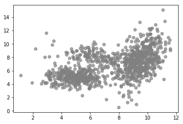
1
2
3
4
5
6
7
8
from latent_variable_models_util import n_true, mu_true, sigma_truefrom latent_variable_models_util import generate_data, plot_data, plot_densities%matplotlib inline X, T = generate_data(n=n_true, mu=mu_true, sigma=sigma_true) plot_data(X, color='grey' )
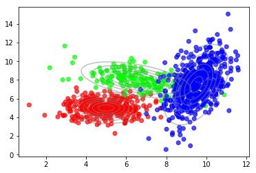
我们可以看到更高密度的集群。此外,与整体分布相比,集群内的分布看起来更像高斯分布。事实上,这些数据是使用下面代码,从三个高斯分布混合生成的,如下图所示。
1
2
plot_data(X, color=T) plot_densities(X, mu=mu_true, sigma=sigma_true)
其背后的概率模型被称为高斯混合模型 (GMM) ,是由 C C C C = 3 C=3 C = 3
p ( x ∣ θ ) = ∑ c = 1 C π c N ( x ∣ μ c , Σ c ) (2) p(\mathbf{x} \lvert \boldsymbol{\theta}) = \sum_{c=1}^{C} \pi_c \mathcal{N}(\mathbf{x} \lvert \boldsymbol{\mu}_c, \boldsymbol{\Sigma}_c)
\tag{2}
p ( x ∣ θ ) = c = 1 ∑ C π c N ( x ∣ μ c , Σ c ) ( 2 )
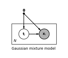
π c \pi_c π c μ c \boldsymbol{\mu}_{c} μ c Σ c \boldsymbol{\Sigma}_{c} Σ c c c c 1 1 1 ∑ c = 1 C π c = 1 \sum_{c=1}^{C} \pi_c = 1 ∑ c = 1 C π c = 1 θ = { π 1 , μ 1 , Σ 1 , … , π C , μ C , Σ C } \boldsymbol{\theta} = \{ \pi_1, \boldsymbol{\mu}_{1}, \boldsymbol{\Sigma}_{1}, \ldots, \pi_C, \boldsymbol{\mu}_{C}, \boldsymbol{\Sigma}_{C} \} θ = { π 1 , μ 1 , Σ 1 , … , π C , μ C , Σ C } t \mathbf{t} t p ( x ∣ t , θ ) p(\mathbf{x} \lvert \mathbf{t}, \boldsymbol{\theta}) p ( x ∣ t , θ ) p ( t ∣ θ ) p(\mathbf{t} \lvert \boldsymbol{\theta}) p ( t ∣ θ ) p ( x , t ∣ θ ) p(\mathbf{x}, \mathbf{t} \lvert \boldsymbol{\theta}) p ( x , t ∣ θ )
p ( x , t ∣ θ ) = p ( x ∣ t , θ ) p ( t ∣ θ ) (3) p(\mathbf{x}, \mathbf{t} \lvert \boldsymbol{\theta}) = p(\mathbf{x} \lvert \mathbf{t}, \boldsymbol{\theta}) p(\mathbf{t} \lvert \boldsymbol{\theta})
\tag{3}
p ( x , t ∣ θ ) = p ( x ∣ t , θ ) p ( t ∣ θ ) ( 3 )
其中 p ( x ∣ t c = 1 , θ ) = N ( x ∣ μ c , Σ c ) p(\mathbf{x} \lvert t_c = 1, \boldsymbol{\theta}) = \mathcal{N}(\mathbf{x} \lvert \boldsymbol{\mu}_c, \boldsymbol{\Sigma} _c) p ( x ∣ t c = 1 , θ ) = N ( x ∣ μ c , Σ c ) p ( t c = 1 ∣ θ ) = π c p(t_c = 1 \lvert \boldsymbol{\theta}) = \pi_c p ( t c = 1 ∣ θ ) = π c t \mathbf{t} t t 2 = 1 t_2 = 1 t 2 = 1 C = 3 C=3 C = 3 t = ( 0 , 1 , 0 ) T \mathbf{t} = (0,1,0)^T t = ( 0 , 1 , 0 ) T p ( x ∣ θ ) p(\mathbf{x} \lvert \boldsymbol{\theta}) p ( x ∣ θ ) t \mathbf{t} t
p ( x ∣ θ ) = ∑ c = 1 C p ( t c = 1 ∣ θ ) p ( x ∣ t c = 1 , θ ) = ∑ c = 1 C π c N ( x ∣ μ c , Σ c ) \begin{align*}
p(\mathbf{x} \lvert \boldsymbol{\theta}) &=
\sum_{c=1}^{C} p(t_c = 1 \lvert \boldsymbol{\theta}) p(\mathbf{x} \lvert t_c = 1, \boldsymbol{\theta}) \\ &=
\sum_{c=1}^{C} \pi_c \mathcal{N}(\mathbf{x} \lvert \boldsymbol{\mu}_c, \boldsymbol{\Sigma}_c)
\tag{4}
\end{align*}
p ( x ∣ θ ) = c = 1 ∑ C p ( t c = 1 ∣ θ ) p ( x ∣ t c = 1 , θ ) = c = 1 ∑ C π c N ( x ∣ μ c , Σ c ) ( 4 )
对于每个观测值值 x i \mathbf{x}_i x i t i \mathbf{t}_i t i
用大写的 X \mathbf{X} X T \mathbf{T} T T \mathbf{T} T 完整数据似然 p ( X , T ∣ θ ) p(\mathbf{X}, \mathbf{T} \lvert \boldsymbol{\theta}) p ( X , T ∣ θ ) θ \boldsymbol{\theta} θ X \mathbf{X} X 边缘似然 (或 不完整的数据似然 ) p ( X ∣ θ ) p(\mathbf{X} \lvert \boldsymbol{\theta}) p ( X ∣ θ )
θ M L E = a r g m a x θ log p ( X ∣ θ ) = a r g m a x θ log ∑ T p ( X , T ∣ θ ) \begin{align*}
\boldsymbol{\theta}_{MLE} &= \underset{\boldsymbol{\theta}}{\mathrm{argmax}} \log p(\mathbf{X} \lvert \boldsymbol{\theta}) \\
&=\underset{\boldsymbol{\theta}}{\mathrm{argmax}} \log \sum_{T} p(\mathbf{X}, \mathbf{T} \lvert \boldsymbol{\theta})
\tag{5}
\end{align*}
θ M L E = θ argmax log p ( X ∣ θ ) = θ argmax log T ∑ p ( X , T ∣ θ ) ( 5 )
上式涉及对数内关于隐变量的累积求和,并且阻碍了对优化问题的解析解。
3. 期望最大算法
虽然无法直接观测到隐变量的值,但我们可以通过似然和先验得到其后验分布。根据贝叶斯定理,我们从一个初步的参数值 θ o l d \boldsymbol{\theta}^{old} θ o l d θ o l d \boldsymbol{\theta}^{old} θ o l d T \mathbf{T} T
p ( T ∣ X , θ o l d ) = p ( X ∣ T , θ o l d ) p ( T ∣ θ o l d ) ∑ T p ( X ∣ T , θ o l d ) p ( T ∣ θ o l d ) (6) p(\mathbf{T} \lvert \mathbf{X}, \boldsymbol{\theta}^{old}) = {
p(\mathbf{X} \lvert \mathbf{T}, \boldsymbol{\theta}^{old}) p(\mathbf{T} \lvert \boldsymbol{\theta}^{old}) \over
\sum_{T} p(\mathbf{X} \lvert \mathbf{T}, \boldsymbol{\theta}^{old}) p(\mathbf{T} \lvert \boldsymbol{\theta}^{old})}
\tag{6}
p ( T ∣ X , θ o l d ) = ∑ T p ( X ∣ T , θ o l d ) p ( T ∣ θ o l d ) p ( X ∣ T , θ o l d ) p ( T ∣ θ o l d ) ( 6 )
依据该后验,我们可以定义完整数据似然 p ( X , T ∣ θ ) p(\mathbf{X}, \mathbf{T} \lvert \boldsymbol{\theta}) p ( X , T ∣ θ )
Q ( θ , θ o l d ) = ∑ T p ( T ∣ X , θ o l d ) log p ( X , T ∣ θ ) = E p ( T ∣ X , θ o l d ) log p ( X , T ∣ θ ) \begin{align*}
\mathcal{Q}(\boldsymbol{\theta}, \boldsymbol{\theta}^{old}) &=
\sum_{T} p(\mathbf{T} \lvert \mathbf{X}, \boldsymbol{\theta}^{old}) \log p(\mathbf{X}, \mathbf{T} \lvert \boldsymbol{\theta}) \\ &=
\mathbb{E}_{p(\mathbf{T} \lvert \mathbf{X}, \boldsymbol{\theta}^{old})} \log p(\mathbf{X}, \mathbf{T} \lvert \boldsymbol{\theta})
\tag{7}
\end{align*}
Q ( θ , θ o l d ) = T ∑ p ( T ∣ X , θ o l d ) log p ( X , T ∣ θ ) = E p ( T ∣ X , θ o l d ) log p ( X , T ∣ θ ) ( 7 )
将该期望作为目标,相对于 θ \boldsymbol{\theta} θ θ n e w \boldsymbol{\theta}^{new} θ n e w
θ n e w = a r g m a x θ Q ( θ , θ o l d ) (8) \boldsymbol{\theta}^{new} = \underset{\boldsymbol{\theta}}{\mathrm{argmax}} \mathcal{Q}(\boldsymbol{\theta}, \boldsymbol{\theta}^{old})
\tag{8}
θ n e w = θ argmax Q ( θ , θ o l d ) ( 8 )
在式 (7) 中,求和是在对数之外进行的,这在 GMM 情形下,使得 θ n e w \boldsymbol{\theta}^{new} θ n e w θ o l d ← θ n e w \boldsymbol{\theta}^{old} \leftarrow \boldsymbol{\theta}^{new} θ o l d ← θ n e w θ \boldsymbol{\theta} θ 期望最大化(EM)算法 的本质。它包括一个计算期望的步骤( E-step ),以更新隐变量的后验;以及一个最大化步骤( M-step ),该步骤依据更新后的隐变量的后验,通过完整数据似然的期望最大化,进一步更新模型参数 θ \boldsymbol{\theta} θ p ( X ∣ θ ) p(\mathbf{X} \lvert \boldsymbol{\theta}) p ( X ∣ θ )
以下小节以更一般的形式描述了 EM 算法。
3.1 一般形式
通过为每个观测 x i \mathbf{x}_i x i t i \mathbf{t}_i t i
log p ( X ∣ θ ) = ∑ i = 1 N log p ( x i ∣ θ ) = ∑ i = 1 N log ∑ c = 1 C p ( x i , t i c = 1 ∣ θ ) \begin{align*}
\log p(\mathbf{X} \lvert \boldsymbol{\theta})
&= \sum_{i=1}^{N} \log p(\mathbf{x}_i \lvert \boldsymbol{\theta}) \\
&= \sum_{i=1}^{N} \log \sum_{c=1}^{C} p(\mathbf{x}_i, t_{ic} = 1 \lvert \boldsymbol{\theta})\tag{9}
\end{align*}
log p ( X ∣ θ ) = i = 1 ∑ N log p ( x i ∣ θ ) = i = 1 ∑ N log c = 1 ∑ C p ( x i , t i c = 1 ∣ θ ) ( 9 )
接下来我们在隐变量 t i \mathbf{t}_i t i q ( t i ) q(\mathbf{t}_i) q ( t i )
log p ( X ∣ θ ) = ∑ i = 1 N log ∑ c = 1 C q ( t i c = 1 ) p ( x i , t i c = 1 ∣ θ ) q ( t i c = 1 ) = ∑ i = 1 N log E q ( t i ) p ( x i , t i ∣ θ ) q ( t i ) \begin{align*}
\log p(\mathbf{X} \lvert \boldsymbol{\theta}) &=
\sum_{i=1}^{N} \log \sum_{c=1}^{C} q(t_{ic} = 1) {p(\mathbf{x}_i, t_{ic} = 1 \lvert \boldsymbol{\theta}) \over q(t_{ic} = 1)} \\ &=
\sum_{i=1}^{N} \log \mathbb{E}_{q(\mathbf{t}_i)} {p(\mathbf{x}_i, \mathbf{t}_i \lvert \boldsymbol{\theta}) \over q(\mathbf{t}_i)}
\tag{10}
\end{align*}
log p ( X ∣ θ ) = i = 1 ∑ N log c = 1 ∑ C q ( t i c = 1 ) q ( t i c = 1 ) p ( x i , t i c = 1 ∣ θ ) = i = 1 ∑ N log E q ( t i ) q ( t i ) p ( x i , t i ∣ θ ) ( 10 )
现在得到一个期望的凹函数 (log \log log Jensen 不等式 来定义 log p ( X ∣ θ ) \log p(\mathbf{X} \lvert \boldsymbol{\theta}) log p ( X ∣ θ ) 下界 L \mathcal{L} L
log p ( X ∣ θ ) = ∑ i = 1 N log E q ( t i ) p ( x i , t i ∣ θ ) q ( t i ) ≥ ∑ i = 1 N E q ( t i ) log p ( x i , t i ∣ θ ) q ( t i ) = E q ( T ) log p ( X , T ∣ θ ) q ( T ) = L ( θ , q ) \begin{align*}
\log p(\mathbf{X} \lvert \boldsymbol{\theta}) &=
\sum_{i=1}^{N} \log \mathbb{E}_{q(\mathbf{t}_i)} {p(\mathbf{x}_i, \mathbf{t}_i\lvert \boldsymbol{\theta}) \over q(\mathbf{t}_i)} \\ &\geq
\sum_{i=1}^{N} \mathbb{E}_{q(\mathbf{t}_i)} \log {p(\mathbf{x}_i, \mathbf{t}_i\lvert \boldsymbol{\theta}) \over q(\mathbf{t}_i)} \\ &=
\mathbb{E}_{q(\mathbf{T})} \log {p(\mathbf{X}, \mathbf{T} \lvert \boldsymbol{\theta}) \over q(\mathbf{T})} \\ &=
\mathcal{L}(\boldsymbol{\theta}, q)
\tag{11}
\end{align*}
log p ( X ∣ θ ) = i = 1 ∑ N log E q ( t i ) q ( t i ) p ( x i , t i ∣ θ ) ≥ i = 1 ∑ N E q ( t i ) log q ( t i ) p ( x i , t i ∣ θ ) = E q ( T ) log q ( T ) p ( X , T ∣ θ ) = L ( θ , q ) ( 11 )
该下界是 θ \boldsymbol{\theta} θ q q q
log p ( X ∣ θ ) − L ( θ , q ) = log p ( X ∣ θ ) − E q ( T ) log p ( X , T ∣ θ ) q ( T ) = E q ( T ) log p ( X ∣ θ ) q ( T ) p ( X , T ∣ θ ) = E q ( T ) log q ( T ) p ( T ∣ X , θ ) = K L ( q ( T ) ∣ ∣ p ( T ∣ X , θ ) ) \begin{align*}
\log p(\mathbf{X} \lvert \boldsymbol{\theta}) - \mathcal{L}(\boldsymbol{\theta}, q) &=
\log p(\mathbf{X} \lvert \boldsymbol{\theta}) - \mathbb{E}_{q(\mathbf{T})} \log {p(\mathbf{X}, \mathbf{T} \lvert \boldsymbol{\theta}) \over q(\mathbf{T})} \\ &=
\mathbb{E}_{q(\mathbf{T})} \log {p(\mathbf{X} \lvert \boldsymbol{\theta}) q(\mathbf{T}) \over p(\mathbf{X}, \mathbf{T} \lvert \boldsymbol{\theta})} \\ &=
\mathbb{E}_{q(\mathbf{T})} \log {q(\mathbf{T}) \over p(\mathbf{T} \lvert \mathbf{X}, \boldsymbol{\theta})} \\ &=
\mathrm{KL}(q(\mathbf{T}) \mid\mid p(\mathbf{T} \lvert \mathbf{X}, \boldsymbol{\theta}))
\tag{12}
\end{align*}
log p ( X ∣ θ ) − L ( θ , q ) = log p ( X ∣ θ ) − E q ( T ) log q ( T ) p ( X , T ∣ θ ) = E q ( T ) log p ( X , T ∣ θ ) p ( X ∣ θ ) q ( T ) = E q ( T ) log p ( T ∣ X , θ ) q ( T ) = KL ( q ( T ) ∣∣ p ( T ∣ X , θ )) ( 12 )
最终得到了 q ( T ) q(\mathbf{T}) q ( T ) p ( T ∣ X , θ ) p(\mathbf{T} \lvert \mathbf{X}, \boldsymbol{\theta}) p ( T ∣ X , θ ) K L KL K L
L ( θ , q ) = log p ( X ∣ θ ) − K L ( q ( T ) ∣ ∣ p ( T ∣ X , θ ) ) (13) \mathcal{L}(\boldsymbol{\theta}, q) = \log p(\mathbf{X} \lvert \boldsymbol{\theta}) - \mathrm{KL}(q(\mathbf{T}) \mid\mid p(\mathbf{T} \lvert \mathbf{X}, \boldsymbol{\theta}))
\tag{13}
L ( θ , q ) = log p ( X ∣ θ ) − KL ( q ( T ) ∣∣ p ( T ∣ X , θ )) ( 13 )
在 EM 算法的 E 步中, 保持 θ \boldsymbol{\theta} θ q q q L ( θ , q ) \mathcal{L}(\boldsymbol{\theta}, q) L ( θ , q ) q q q
q n e w = a r g m a x q L ( θ o l d , q ) = a r g m i n q K L ( q ( T ) ∣ ∣ p ( T ∣ X , θ o l d ) ) \begin{align*}
q^{new} &=
\underset{q}{\mathrm{argmax}} \mathcal{L}(\boldsymbol{\theta}^{old}, q) \\ &=
\underset{q}{\mathrm{argmin}} \mathrm{KL}(q(\mathbf{T}) \mid\mid p(\mathbf{T} \lvert \mathbf{X}, \boldsymbol{\theta}^{old}))
\tag{14}
\end{align*}
q n e w = q argmax L ( θ o l d , q ) = q argmin KL ( q ( T ) ∣∣ p ( T ∣ X , θ o l d )) ( 14 )
L ( θ , q ) \mathcal{L}(\boldsymbol{\theta}, q) L ( θ , q ) KL ( q ( T ) ∣ ∣ p ( T ∣ X , θ ) ) \text{KL}(q(\mathbf{T}) \mid\mid p(\mathbf{T} \lvert \mathbf {X}, \boldsymbol{\theta})) KL ( q ( T ) ∣∣ p ( T ∣ X , θ )) log p ( X ∣ θ ) \log p(\mathbf{X} \lvert \boldsymbol{\theta}) log p ( X ∣ θ ) q q q
如果能够获得真实的后验,就像在 GMM 的情况下一样,可以将 q ( T ) q(\mathbf{T}) q ( T ) p ( T ∣ X , θ ) p(\mathbf{T} \lvert \mathbf{X}, \boldsymbol{\theta} ) p ( T ∣ X , θ ) K L KL K L 0 0 0 变分推断 ,它使用特定形式的 q q q q q q q q q K L KL K L
在 M 步中,保持 q q q θ \boldsymbol{\theta} θ L ( θ , q ) \mathcal{L}(\boldsymbol{\theta}, q) L ( θ , q ) θ \boldsymbol{\theta} θ
θ n e w = a r g m a x θ L ( θ , q n e w ) = a r g m a x θ E q n e w ( T ) log p ( X , T ∣ θ ) q n e w ( T ) = a r g m a x θ E q n e w ( T ) log p ( X , T ∣ θ ) − E q n e w ( T ) log q n e w ( T ) = a r g m a x θ E q n e w ( T ) log p ( X , T ∣ θ ) + c o n s t . \begin{align*}
\boldsymbol{\theta}^{new} &=
\underset{\boldsymbol{\theta}}{\mathrm{argmax}} \mathcal{L}(\boldsymbol{\theta}, q^{new}) \\ &=
\underset{\boldsymbol{\theta}}{\mathrm{argmax}} \mathbb{E}_{q^{new}(\mathbf{T})} \log {p(\mathbf{X}, \mathbf{T} \lvert \boldsymbol{\theta}) \over q^{new}(\mathbf{T})} \\ &=
\underset{\boldsymbol{\theta}}{\mathrm{argmax}} \mathbb{E}_{q^{new}(\mathbf{T})} \log p(\mathbf{X}, \mathbf{T} \lvert \boldsymbol{\theta}) - \mathbb{E}_{q^{new}(\mathbf{T})} \log q^{new}(\mathbf{T}) \\ &=
\underset{\boldsymbol{\theta}}{\mathrm{argmax}} \mathbb{E}_{q^{new}(\mathbf{T})} \log p(\mathbf{X}, \mathbf{T} \lvert \boldsymbol{\theta}) +\mathrm{const.}
\tag{15}
\end{align*}
θ n e w = θ argmax L ( θ , q n e w ) = θ argmax E q n e w ( T ) log q n e w ( T ) p ( X , T ∣ θ ) = θ argmax E q n e w ( T ) log p ( X , T ∣ θ ) − E q n e w ( T ) log q n e w ( T ) = θ argmax E q n e w ( T ) log p ( X , T ∣ θ ) + const. ( 15 )
如果真正的后验是已知的, 则式 (15) 变为式 (7) ,除了在优化过程中可以忽略的常数项。同样,让 θ o l d ← θ n e w \boldsymbol{\theta}^{old} \leftarrow \boldsymbol{\theta}^{new} θ o l d ← θ n e w
4. 高斯混合模型的期望最大化算法
The parameters for a GMM with 3 components are θ = { π 1 , μ 1 , Σ 1 , π 2 , μ 2 , Σ 2 , π 3 , μ 3 , Σ 3 } \boldsymbol{\theta} = \{ \pi_1, \boldsymbol{\mu}_{1}, \boldsymbol{\Sigma}_{1}, \pi_2, \boldsymbol{\mu}_{2}, \boldsymbol{\Sigma}_{2}, \pi_3, \boldsymbol{\mu}_{3}, \boldsymbol{\Sigma}_{3} \} θ = { π 1 , μ 1 , Σ 1 , π 2 , μ 2 , Σ 2 , π 3 , μ 3 , Σ 3 } c c c p ( t c = 1 ∣ θ ) = π c p(t_c = 1 \lvert \boldsymbol{\theta}) = \pi_c p ( t c = 1 ∣ θ ) = π c x \mathbf{x} x p ( x ∣ t c = 1 , θ ) = N ( x ∣ μ c , Σ c ) p(\mathbf{x} \lvert t_c = 1, \boldsymbol{\theta}) = \mathcal{N}(\mathbf{x} \lvert \boldsymbol{\mu}_c, \boldsymbol{\Sigma}_c) p ( x ∣ t c = 1 , θ ) = N ( x ∣ μ c , Σ c )
具有 3 个组份的 GMM 模型参数是 θ = { π 1 , μ 1 , Σ 1 , p i 2 、 μ 2 、 Σ 2 、 π 3 、 μ 3 、 Σ 3 } \boldsymbol{\theta} = \{ \pi_1, \boldsymbol{\mu}_{1}, \boldsymbol{\Sigma}_{1}, \ pi_2、\boldsymbol{\mu}_{2}、\boldsymbol{\Sigma}_{2}、\pi_3、\boldsymbol{\mu}_{3}、\boldsymbol{\Sigma }_{3} \} θ = { π 1 , μ 1 , Σ 1 , p i 2 、 μ 2 、 Σ 2 、 π 3 、 μ 3 、 Σ 3 } c c c p ( t c = 1 ∣ θ ) = π c p(t_c = 1 \lvert \boldsymbol{\theta}) = \pi_c p ( t c = 1 ∣ θ ) = π c x \mathbf{x} x
4.1 numpy 和 scipy 的实现
1
2
3
import numpy as npfrom scipy.stats import multivariate_normal as mvn
在 E 步中,使用式( 6 )将隐变量的近似后验 q ( T ) q(\mathbf{T}) q ( T ) p ( T ∣ X , θ ) p(\mathbf{T} \lvert \mathbf{X}, \boldsymbol{\theta}) p ( T ∣ X , θ )
1
2
3
4
5
6
7
8
9
10
11
12
13
14
15
16
17
18
19
20
21
22
def e_step (X, pi, mu, sigma ): """ Computes posterior probabilities from data and parameters. Args: X: observed data (N, D). pi: prior probabilities (C,). mu: mixture component means (C, D). sigma: mixture component covariances (C, D, D). Returns: Posterior probabilities (N, C). """ N = X.shape[0 ] C = mu.shape[0 ] q = np.zeros((N, C)) for c in range (C): q[:, c] = mvn(mu[c], sigma[c]).pdf(X) * pi[c] return q / np.sum (q, axis=-1 , keepdims=True )
在 M 步中,取 L ( θ , q ) \mathcal{L}(\boldsymbol{\theta}, q) L ( θ , q ) π c \pi_c π c μ c \boldsymbol{\mu}_{c} μ c Σ c \boldsymbol{\Sigma}_{c} Σ c 0 0 0 ∑ c = 1 C π c = 1 \sum_{c=1}^C \pi_c = 1 ∑ c = 1 C π c = 1 Σ c ) T \boldsymbol{\Sigma}_{c})^T Σ c ) T
π c = 1 N ∑ i = 1 N q ( t i c = 1 ) (16) \pi_c = {1 \over N} \sum_{i=1}^N q(t_{ic} = 1) \tag{16}
π c = N 1 i = 1 ∑ N q ( t i c = 1 ) ( 16 )
μ c = ∑ i = 1 N q ( t i c = 1 ) x i ∑ i = 1 N q ( t i c = 1 ) (17) \boldsymbol{\mu}_{c} = {\sum_{i=1}^N q(t_{ic} = 1) \mathbf{x}_i \over \sum_{i=1}^N q(t_{ic} = 1)} \tag{17}
μ c = ∑ i = 1 N q ( t i c = 1 ) ∑ i = 1 N q ( t i c = 1 ) x i ( 17 )
Σ c = ∑ i = 1 N q ( t i c = 1 ) ( x i − μ c ) ( x i − μ c ) T ∑ i = 1 N q ( t i c = 1 ) (18) \boldsymbol{\Sigma}_{c} = {\sum_{i=1}^N q(t_{ic} = 1) (\mathbf{x}_i - \boldsymbol{\mu}_{c}) (\mathbf{x}_i - \boldsymbol{\mu}_{c})^T \over \sum_{i=1}^N q(t_{ic} = 1)} \tag{18}
Σ c = ∑ i = 1 N q ( t i c = 1 ) ∑ i = 1 N q ( t i c = 1 ) ( x i − μ c ) ( x i − μ c ) T ( 18 )
1
2
3
4
5
6
7
8
9
10
11
12
13
14
15
16
17
18
19
20
21
22
23
24
25
26
27
28
29
30
31
def m_step (X, q ): """ Computes parameters from data and posterior probabilities. Args: X: data (N, D). q: posterior probabilities (N, C). Returns: tuple of - prior probabilities (C,). - mixture component means (C, D). - mixture component covariances (C, D, D). """ N, D = X.shape C = q.shape[1 ] sigma = np.zeros((C, D, D)) pi = np.sum (q, axis=0 ) / N mu = q.T.dot(X) / np.sum (q.T, axis=1 , keepdims=True ) for c in range (C): delta = (X - mu[c]) sigma[c] = (q[:, [c]] * delta).T.dot(delta) / np.sum (q[:, c]) return pi, mu, sigma
为了计算下界,使用 E 步和 M 步的结果,首先重排公式 (11) :
L ( θ , q ) = ∑ i = 1 N E q ( t i ) log p ( x i , t i ∣ θ ) q ( t i ) \mathcal{L}(\boldsymbol{\theta}, q) = \sum_{i=1}^{N} \mathbb{E}_{q(\mathbf{t}_i)} \log {p(\mathbf{x}_i, \mathbf{t}_i \lvert \boldsymbol{\theta}) \over q(\mathbf{t}_i)}
L ( θ , q ) = i = 1 ∑ N E q ( t i ) log q ( t i ) p ( x i , t i ∣ θ )
= ∑ i = 1 N ∑ c = 1 C q ( t i c = 1 ) log p ( x i , t i c = 1 ∣ θ ) q ( t i c = 1 ) =\sum_{i=1}^{N} \sum_{c=1}^{C} q(t_{ic} = 1) \log {p(\mathbf{x}_i, t_{ic} = 1 \lvert \boldsymbol{\theta}) \over q(t_{ic} = 1)}
= i = 1 ∑ N c = 1 ∑ C q ( t i c = 1 ) log q ( t i c = 1 ) p ( x i , t i c = 1 ∣ θ )
= ∑ i = 1 N ∑ c = 1 C q ( t i c = 1 ) { log p ( x i ∣ t i c = 1 , θ ) + log p ( t i c = 1 ∣ θ ) − log q ( t i c = 1 ) } (19) =\sum_{i=1}^{N} \sum_{c=1}^{C} q(t_{ic} = 1) \{ \log p(\mathbf{x}_i \lvert t_{ic} = 1, \boldsymbol{\theta}) + \log p(t_{ic} = 1 \lvert \boldsymbol{\theta}) - \log q(t_{ic} = 1) \} \tag{19}
= i = 1 ∑ N c = 1 ∑ C q ( t i c = 1 ) { log p ( x i ∣ t i c = 1 , θ ) + log p ( t i c = 1 ∣ θ ) − log q ( t i c = 1 )} ( 19 )
然后以如下形式实现它:
1
2
3
4
5
6
7
8
9
10
11
12
13
14
15
16
17
18
19
20
21
22
def lower_bound (X, pi, mu, sigma, q ): """ Computes lower bound from data, parameters and posterior probabilities. Args: X: observed data (N, D). pi: prior probabilities (C,). mu: mixture component means (C, D). sigma: mixture component covariances (C, D, D). q: posterior probabilities (N, C). Returns: Lower bound. """ N, C = q.shape ll = np.zeros((N, C)) for c in range (C): ll[:,c] = mvn(mu[c], sigma[c]).logpdf(X) return np.sum (q * (ll + np.log(pi) - np.log(np.maximum(q, 1e-8 ))))
模型训练交替迭代 E 步和 M 步,直到下界收敛。为了增加逃出局部最大值并找到全局最大值的机会,会随机初始化参数并重新训练多次。
1
2
3
4
5
6
7
8
9
10
11
12
13
14
15
16
17
18
19
20
21
22
23
24
25
26
27
28
29
30
31
32
33
34
35
36
37
38
39
40
41
42
43
44
45
46
def random_init_params (X, C ): D = X.shape[1 ] pi = np.ones(C) / C mu = mvn(mean=np.mean(X, axis=0 ), cov=[np.var(X[:, 0 ]), np.var(X[:, 1 ])]).rvs(C).reshape(C, D) sigma = np.tile(np.eye(2 ), (C, 1 , 1 )) return pi, mu, sigma def train (X, C, n_restarts=10 , max_iter=50 , rtol=1e-3 ): q_best = None pi_best = None mu_best = None sigma_best = None lb_best = -np.inf for _ in range (n_restarts): pi, mu, sigma = random_init_params(X, C) prev_lb = None try : for _ in range (max_iter): q = e_step(X, pi, mu, sigma) pi, mu, sigma = m_step(X, q) lb = lower_bound(X, pi, mu, sigma, q) if lb > lb_best: q_best = q pi_best = pi mu_best = mu lb_best = lb if prev_lb and np.abs ((lb - prev_lb) / prev_lb) < rtol: break prev_lb = lb except np.linalg.LinAlgError: pass return pi_best, mu_best, sigma_best, q_best, lb_best pi_best, mu_best, sigma_best, q_best, lb_best = train(X, C=3 ) print (f'Lower bound = {lb_best:.2 f} ' )
Lower bound = -3923.77
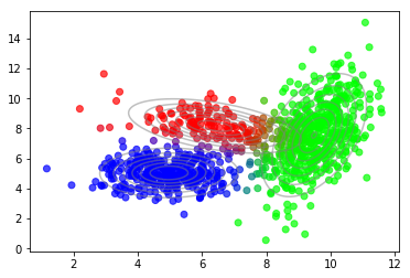
收敛后,我们可以使用隐变量的后验来绘制数据点到组份的软分配。
1
2
plot_data(X, color=q_best) plot_densities(X, mu=mu_best, sigma=sigma_best)
4.2 最优的组份数量
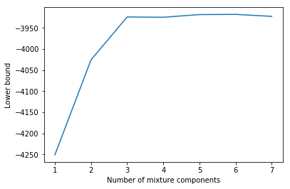
Usually, we do not know the optimal number of mixture components a priori. But we can get a hint when plotting the lower bound vs. the number of mixture components.
通常,我们无法先验地知道混合组份的最佳数量。但当绘制下界与混合组份数关系时,可以得到一些提示。
1
2
3
4
5
6
7
8
9
10
11
12
import matplotlib.pyplot as pltCs = range (1 , 8 ) lbs = [] for C in Cs: lb = train(X, C)[-1 ] lbs.append(lb) plt.plot(Cs, lbs) plt.xlabel('Number of mixture components' ) plt.ylabel('Lower bound' );
在到达 C = 3 C = 3 C = 3
确定最佳组份数量的更原则性方法需要对模型参数进行贝叶斯处理。在这种情况下,下界将考虑模型复杂性,我们会看到 C > 3 C \gt 3 C > 3 C = 3 C = 3 C = 3 [1]
4.3 scikit-learn 实现
上面的初级实现仅用于说明目的。 Scikit-learn 已经附带了一个可以轻松使用的“GaussianMixture” 类。
1
2
3
4
5
6
7
from sklearn.mixture import GaussianMixturegmm = GaussianMixture(n_components=3 , n_init=10 ) gmm.fit(X) plot_data(X, color=gmm.predict_proba(X)) plot_densities(X, mu=gmm.means_, sigma=gmm.covariances_)
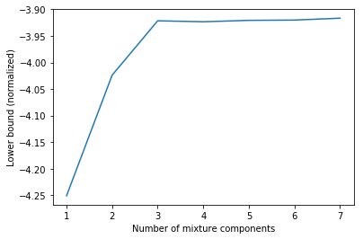
结果非常相似。差异来自不同的随机初始化方法。此外,对下界与组份数量关系的绘图,再现了之前的发现。
1
2
3
4
5
6
7
8
9
10
11
Cs = range (1 , 8 ) lbs = [] for C in Cs: gmm = GaussianMixture(n_components=C, n_init=10 ) gmm.fit(X) lbs.append(gmm.lower_bound_) plt.plot(Cs, lbs) plt.xlabel('Number of mixture components' ) plt.ylabel('Lower bound (normalized)' );
在这个例子中,通过gmm.lower_bound_ 获得的下界值做了归一化,即除以 N = 1000 N = 1000 N = 1000
5 结论
GMM 中隐变量的推断和参数估计是精确推断的一个例子。精确的后验可以在 E 步中获得,并且在 M 步中存在参数 MLE 的解析解。但是对于许多实际感兴趣的模型,精确推断基本不可能,必须使用近似推断方法。 变分推断 就是其中之一,将在下一篇隐变量模型的文章中进行介绍,并附上一个 变分自动编码器 作为应用示例。
References
[1] Christopher M. Bishop. [Pattern Recognition and Machine Learning](http://www.springer.com/de/book/9780387310732) ([PDF](https://www.microsoft.com/en-us/research/uploads/prod/2006/01/Bishop-Pattern-Recognition-and-Machine-Learning-2006.pdf)), Chapter 9. [2] Kevin P. Murphy. [Machine Learning, A Probabilistic Perspective](https://mitpress.mit.edu/books/machine-learning-0), Chapter 11.