🔥 自回归条件神经过程

【摘 要】 条件神经过程（CNP）是一种具有吸引力的元学习模型，它可以产生经过良好校准的预测，并且可以通过最大似然程序进行训练。尽管条件神经过程有很多优势，但 其无法在预测中建立依赖关系模型 。已经有多项工作为此提出了解决方案，但都以 近似 或 仅限于高斯 预测为代价的。在本文工作中，我们建议不对条件神经过程模型或训练过程进行任何修改，而是改变其在测试时的部署方式。我们从 神经自回归密度估计器 (NADE) 文献中汲取了灵感，使用 概率链式法则 自回归地定义联合预测分布，而不是对每个目标点进行独立的预测。实验结果表明，此过程允许 因子化的高斯条件神经过程 对相关的、非高斯的预测分布进行建模。令人惊讶的是，在使用合成数据和真实数据的广泛任务中，我们表明自回归模式下的条件神经过程，不仅显著优于非自回归条件神经过程，而且还与更复杂的模型（训练成本和难度可能高得多）形成了竞争关系。自回归条件神经过程性能出色的原因在于：不需要通过训练来模拟联合分布的依赖性。我们的工作提供了一个示例，说明了神经过程能够从 “神经分布估计的思想” 中受益，进而可以推动对其他神经过程模型的自回归部署研究。

【原 文】 Bruinsma, W. 等 (2023) ‘Autoregressive conditional neural processes’, in The eleventh international conference on learning representations. Available at: https://openreview.net/forum?id=OAsXFPBfTBh.

【单 位】 微软 AI4 科学研究院；剑桥大学；英国南极调查局；艾伦图灵研究所

1 引言

条件神经过程 (CNP; Garnelo 等, 2018a ^[27]) 是一个元学习模型族，它结合了深度学习的灵活性和概率模型的不确定性感知能力。条件神经过程可以采用简单的最大似然程序进行训练，并能够生成经过良好校准的预测，并且可以自然地处理离网和缺失数据。这使它们非常适合气候科学和医疗保健中的任务。自引入条件神经过程以来，还提出了注意力（ACNP；Kim 等，2019 ^[46]）和卷积（ConvCNP；Gordon 等，2020 ^[33]）等变体。

不幸的是，现有条件神经过程无法对统计依赖性建模（见 图(1) 左），这影响了其预测性能，此外，该方法无法抽取出下游估计任务所需的 相干样本（Markou 等，2022 ^[61]）。

已经有人提出了多种方法来解决此问题。

• Garnelo 等 (2018b ^[28]) 介绍了隐神经过程 (LNP)，它使用隐变量来归纳依赖性和模型的非高斯性。这种做法使似然很难处理，只能实施近似推断。
• 完全卷积高斯神经过程也是一种解决方案（FullConvGNP；Bruinsma 等，2021 ^[8]），但它仅允许高斯预测以保持易处理性。全卷积神经过程使用神经网络来定义了预测高斯过程的均值函数和协方差函数，但神经网络架构比较复杂，并且实际上只适用于一维输入，这限制了其使用。
• Markou 等 (2022 ^[61]) 提出了高斯神经过程 (GNP)，该模型相当简单，但相对于全卷积神经过程 来说牺牲了部分性能。

图 1：在随机的锯齿状函数上训练并应用于标准模式下的 ConvCNP（左）；应用于本文提出的自回归 (AR) 模式下的 ConvCNP（右）。黑色十字表示观测数据，蓝线表示模型抽取的样本，底部图对应于上图中垂直虚线标记位置处的边缘预测分布。在标准模式下，CNP 使用独立的高斯分布（左）对每个输出进行建模。然而，在自回归模式下，同一个条件神经过程可以产生连贯的样本和多峰分布（右）。

在本文中，我们提出了一种更简单的方法来对神经过程的依赖关系进行建模，这就是 自回归 (AR) 采样 。

自回归采样不需要更改架构或训练过程，只是改变了条件神经过程在测试时的部署方式，提取了一些通常会被放弃的预测信息。我们并不同时对所有目标点进行预测，而是将自回归的样本反馈到模型中。自回归条件神经过程为了 “实现非高斯预测和相关预测” 而放弃了 “边缘化和重排列下的一致性”（这是许多神经过程模型的基础）。在 表(1) 中，我们将自回归条件神经过程置于其他神经过程模型的架构中。

我们的主要贡献是：

• 我们表明，自回归模式中使用的条件神经过程，能够捕获丰富的非高斯预测分布并生成相关样本（ 图(1)右 ）。这是不可思议的的，因为这些条件神经过程只具有高斯似然，并未经过训练来模拟联合分布的依赖性或非高斯性，而且训练成本明显低于 隐神经过程 和 全卷积神经过程 （ 图(2) ）。

• 我们证明，如果有足够的数据和模型容量， 自回归条件神经过程 的性能至少与 高斯神经过程 的性能相当，后者在其预测中显式建模了相关性。

• 通过将自回归条件神经过程视为一种神经密度估计器（Uria 等，2016 年^[85]），我们展现了其与深度生成建模文献中一系列现有方法之间的联系。

• 在范围广泛的高斯和非高斯回归任务中，自回归条件神经过程在预测对数似然方面始终与所有其他神经过程模型之间竞争，而且通常明显优于所有其他神经过程模型。

• 我们将自回归条件神经过程部署到涉及真实世界气候数据的一系列任务中。为了用计算上易于处理的方式处理高分辨率数据，我们为 ConvCNP 引入了一种新颖的多尺度架构。我们还将自回归 ConvCNP 与 贝塔-类别混合分布的似然相结合，并且与其他神经过程相比产生了更好的结果。

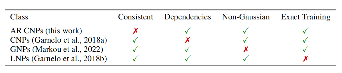
表 1：各种类型神经过程的比较。展示了某个类型的预测是否具备一致性、依赖性、非高斯性，以及是否可以在不逼近目标函数的情况下进行训练。对于条件神经过程来说，实现非高斯输出很容易（即使 Garnelo 等 (2018a) 对其作出了高斯预测的假设）；但对于高斯神经过程来说并非如此。

图 2：非高斯锯齿数据的负对数似然。在自回归模式下部署 ConvCNP 可显着提高性能，并优于具有高斯 (FullConvGNP) 和非高斯 (ConvLNP) 预测分布的最先进的神经过程，而训练成本仅为其一小部分。

2 自回归条件神经过程

（1）元学习

我们首先定义问题设置。设 $\mathcal{X}$ 为紧致输入空间， $\mathcal{Y}$ 为输出空间。设 $\mathcal{D}_N = (\mathcal{ X \times Y})^N$ 是所有 $N$ 个输入-输出对集合的集合，并设 $\mathcal{D} = \bigcup^{\infty}_{N=0} \mathcal{D}_N$ 。我们称元素 $D \in \mathcal{D}$ 为数据集并将其表示为 $D = (\mathbf{x, y})$，其中 $\mathbf{x} \in \mathcal{X}^N$ , $\mathbf{y} \in \mathcal{Y}^N$ 分别是输入和输出。

在元学习中，我们得到一组数据集 $(D_m)^{M}_{m=1}$，被称为元数据集，单个数据集 $D_m$ 被称为任务（Vinyals 等，2016 ^[88]）。每个任务 $D_m$ 可以被拆分为两部分 $D_m = D^{(c)}_m \cup D^{(t)}_m$ ，其中 $D^{(c)}_m = (\mathbf{x}^{(c)}_m , \mathbf{y}^{(c)}_m )$ 为背景集，$D^{(t)}_m = (x^{(t)}_m, y^{(t)}_m)$ 为目标集。同时，称 $\mathbf{x}^{(c)}_m$ 为背景输入， $\mathbf{y}^{(c)}_m$ 为背景输出，称 $\mathbf{x}^{(t)}_m$ 目标输入，$\mathbf{y}^{(t)}_m$ 为目标输出。

我们的目标是： 设计一种使用背景集 $D^{(c)}_m$ 的算法，在给定目标输入 $x^{(t)}_m$ 的情况下，为目标输出 $y^{(t)}_m$ 生成最佳可能预测。

（2）神经过程

令 $\mathcal{P}$ 表示在 $\mathcal{X}$ 上的、值域为 $\mathcal{Y}$ 的所有随机过程构成的集合。一些主要的神经过程之间主要区别如下：

神经过程 (NP)：指所有直接地、灵活地参数化映射 $\pi_{\theta} : \mathcal{D} \rightarrow \mathcal{Q}$，其中 $\mathcal{Q} \subseteq \mathcal{P}$，$\theta$ 是可学习的参数。

条件神经过程（CNP）：将神经过程中的 $\mathcal{Q}$ 约束为高斯过程 $f$ 的集合，但对于任意 $x \neq y$，有 $\mathrm{cov}(f(x), f(y)) = 0$。

高斯神经过程（GNP）： 将 $\mathcal{Q}$ 约束为连续高斯过程的集合。

隐神经过程（LNP）：通过使用隐变量，使 $\mathcal{Q}$ 成为非高斯过程的集合 (Garnelo 等, 2018b ^[28]) 。

如果令 $P_{\mathbf{x}^{(t)}_m} \pi(D^{(c)}_m)$ 表示在 $\mathbf{x}^{(t)}_m$ 处计算的随机过程 $\pi(D^{(c)}_m )$ 的有限维分布，并将其密度表示为 $q_{\theta}( \bullet | \mathbf{x}^{(t)}_m，D^{(c)}_m)$ 。为了学习参数 $\theta$ ，神经过程将寻求最大化如下似然：

$$\mathcal{L}_M(\pi) = \frac{1}{M} \sum^{M}_{m=1} \log q_{\theta}(\mathbf{y}^{(t)}_m | \mathbf{x}^{(t)}_m, D^{(c)}_m ) \tag{1}$$

对于 条件神经过程 和 高斯神经过程，$\mathcal{L}_M$ 可以精确计算，因为 $q_{\theta}$ 是高斯的。但对于隐神经过程，$\mathcal{L}_M$ 只能近似计算（Garnelo 等，2018b ^[28]；Foong 等，2020 ^[25]），这通常会影响计算性能。

（3）自回归条件神经过程

我们的建议是： 采用现有条件神经过程并以自回归方式运行它 ，即将过去输出的预测反馈回模型。受乘法规则启发，我们将联合预测定义为条件分布之积，然后用条件神经过程对每个条件分布建模。例如，在三个目标点的情况下，有

$$q_{\theta}(y^{(t)}_1,y^{(t)}_2,y^{(t)}_3 | D^{(c)}_m) = q_{\theta}(y^{(t)}_3 | \mathbf{y}^{(t)}_{1:2}, D^{(c)}_m)\,q_{\theta}(y^{(t)}_2 | y^{(t)}_1 , D^{(c)}_m) \,q_{\theta}(y^{(t)}_1 | D^{(c)}_m)$$

为了能够对上述方法进行理论分析，我们着手建立一些更正式的符号表示：假设 $\pi_{\theta} : \mathcal{D} \rightarrow \mathcal{Q}$ 代表一个神经过程，我们希望在给定背景集 $D^{(c)}$ 时，在某些目标输入 $\mathbf{x}^{(t)}$ 处进行预测。标准神经过程应当输出预测性的 $P_{\mathbf{x}^{(t)}} (\pi_{\theta}D^{(c)})$。对于条件神经过程而言，$P_{\mathbf{x}^{(t)}} (\pi_{\theta}D^{(c)})$ 是一个因子化的高斯分布。

我们建议采用 程序 2.1 所述的方式，自回归地滚动输出神经过程。

【程序 2.1（神经过程的自回归应用）】

对于神经过程 $\pi_{\theta}$ 、背景集 $D^{(c)} = (\mathbf{x}^{(c)}, \mathbf{y}^{(c)})$ 和目标输入 $\mathbf{x}^{(t)}$ ，令 $\mathrm{AR}_{\mathbf{x}^{(t)}} (\pi_{\theta}, D^{(c)})$ 为下式定义的分布：

$$\quad \text{for} \quad i = 1, \ldots, N \text{,} \quad , y^{(t)}_i \sim P_{x^{(t)}_i} \pi_{\theta} (\mathbf{x}^{(c)} \oplus \mathbf{x}^{(t)}_{1:(i−1)}, \mathbf{y}^{(c)} \oplus \mathbf{y}^{(t)}_{1:(i−1)}) \tag{2}$$

其中 $\mathbf{a \oplus b}$ 连接（concatenates）两个向量 $\mathbf{a}$ 和 $\mathbf{b}$ 。有关说明，请参见附录 C 中的 图(7) 。

由于较早的样本 $y^{(t)}_i$ 会被反馈到 $\pi_{\theta}$ 的新应用中，因此整个样本 $\mathbf{y}^{(t)}$ 之间具有了相关性，即便 $\pi_{\theta}$ 像条件神经过程那样并不直接对目标输出之间的依赖性建模。在测试时，计算 $\mathbf{y}^{(t)}$ 对应的 $\mathrm{AR}_{\mathbf{x}^{(t)}} (\pi_{\theta}, D^{(c)})$ 的密度 $q^{(AR)}_\theta$ 可以使用公式：

$$\log q^{(AR)}_{\theta} (\mathbf{y}^{(t)} | \mathbf{x}^{(t)}, D^{(c)}) = \sum\limits^{N}_{i=1} \log q_{\theta} \left(y^{(t)}_i | x^{(t)}_i , D^{(c)} \oplus (\mathbf{x}^{(t)}_{1:(i−1)}, \mathbf{y}^{(t)}_{1:(i−1)}) \right) \tag{3}$$

虽然任何神经过程都可以用于自回归，但我们比较关注条件神经过程，因为其计算成本最低。

（4）理解无限数据的极限情况

为了更好地理解为什么自回归条件神经过程能够成功地对依赖关系进行建模，我们分析了无限数据和模型容量的理想化情况。令 $p(f)$ 表示生成数据的随机过程的规则，令 $p(\varepsilon)$ 表示产生观测噪声的随机过程的规则，且令向量 $\mathbf{x}$ 的 i.i.d. 噪声向量为 $\varepsilon(\mathbf{x})$。我们假设

$$\mathbf{y}^{(c)}_m = y_m(\mathbf{x}^{(c)}_m ) \quad \text{并且} \quad \mathbf{y}^{(t)}_m = y_m(\mathbf{x}^{(t)}_m) \quad \text{其中} \quad y_m( \bullet ) = f_m( \bullet ) + \varepsilon_m( \bullet )\tag{4}$$

$(f_m)^{M}_{m=1}$ 是从 $p(f)$ 中 i.i.d. 抽取的，并且 $(\varepsilon_m)^{M}_{m=1}$ 是从 $p(\varepsilon)$ 中 i.i.d. 抽取的。将预测映射 $\pi_y : \mathcal{D} \rightarrow \mathcal{P}$ 定义为从某个数据集到 $y$ 上后验的映射，即 $\pi_y(D) = p(y|D)$。然后 $\mathcal{L}_M$ 是以下无限样本目标的蒙特卡罗近似（Foong 等，2020）：

$$L_{\infty} (\pi) = − \mathbb{E}_{p(D^{(c)}) p(\mathbf{x}^{(t)})}\left[\mathrm{KL}(P_{\mathbf{x}^{(t)}} \pi_y(D^{(c)}), P_{\mathbf{x}^{(t)}} \pi(D^{(c)})) \right] + \quad \text{const} \tag{5}$$

在适当的正则假设下，当期望的 KL 散度项为零时， $L_{\infty} (\pi)$ 在所有 $\pi$ 上最大化，并且当且仅当 $\pi = \pi_y$ 时才会发生这种情况。在实际工作中，神经过程不会在所有 $\pi$ 上最大化 $L_{\infty} (\pi)$ ，而是 (i) 使用有限大小的元数据集和 (ii) 限制 $\mathcal{Q} \subseteq \mathcal{P}$ ：

$$\overbrace{\pi_M \in \underset{\mathrm{all} \, \pi: \mathcal{D} \rightarrow \mathcal{Q}}{\arg \max} \mathcal{L}_M(\pi)}^{实际计算的} \xrightarrow[M \rightarrow \infty ]{(i)} \overbrace{\pi_{\infty } \in \underset{\mathrm{all} \, \pi: \mathcal{D} \rightarrow \mathcal{Q}}{\arg \max} \mathcal{L}_{\infty }(\pi)}^{理想的神经过程} \xrightarrow[\mathcal{Q} \rightarrow \mathcal{P} ]{(ii)} \overbrace{\pi_{y} \in \underset{\mathrm{all} \, \pi: \mathcal{D} \rightarrow \mathcal{Q}}{\arg \max} \mathcal{L}_{\infty}(\pi)}^{精确的预测映射} \tag{6}$$

这里的 $\pi_M$ 是在 式 (1) 的实际目标上训练的神经过程，在无限数据限制下，近似于理想神经过程 $\pi_{\infty}$ 。理想神经过程取决于 $\mathcal{Q}$ 的选择，即正在考虑的神经过程类别，并且反过来近似于 $\pi_y$ 。对于 条件神经过程 和 高斯神经过程 ，利用在 $q$ 上最小化 $\mathrm{KL}(p, q)$ 会匹配矩的事实 (Minka, 2001) ，我们可以很容易地确定甚至计算这两类神经过程的理想神经过程。

• 理想的条件神经过程 会预测一个对角协方差的高斯过程，其均值函数和边缘方差函数与 $\pi_y : \pi_{\infty}(D) = \mathcal{GP}(m, k)$ 匹配，其中 $m(x) = \mathbb{E}[y(x) | D]$, $k(x, x') = \mathbb{V}[y(x) | D]$，且当 $x = x'$ 时有 $k(x, x') = 0$。

• 理想的高斯神经过程 会预测一个全协方差的高斯过程，其均值函数和协方差与 $\pi_y ： \pi_{\infty}(D) = GP(m, k)$ 匹配，其中 $m(x) = \mathbb{E}[y(x) | D]$ , $k(x, x') = \mathrm{cov}(y(x), y(x') | D)$ 。

本小节的主要结论： 理想的条件神经过程（不管是否建模了相关性），在自回归模式下部署时都会变得优于理想的高斯过程。

【命题 2.1（自回归条件神经过程相对于高斯神经过程的优势）】

在 $y$ 上假设适当的正则性条件。设 $\pi_C$ 为理想的条件神经过程， $\pi_G$ 为理想的高斯神经过程。然后，对于所有输入 $\mathbf{x}$ 和数据集 $D \in \mathcal{D}$ ，

$$\mathrm{KL}\left(P_{\mathbf{x}} \pi_y(D), \mathrm{AR}_{\mathbf{x}}\left(\pi_{\mathrm{C}}, D\right)\right) \leq \mathrm{KL}\left(P_{\mathbf{x}} \pi_y(D), P_{\mathbf{x}} \pi_{\mathrm{G}}(D)\right) \tag{7}$$

我们在 附录 A 中提供了一个证明。直观地说，自回归条件神经过程的优势来自于其对非高斯依赖性进行建模的能力。 命题 2.1 表明，要想优于高斯神经过程，只需训练条件神经过程对 $\pi_y$ 的边缘进行建模，并依靠自回归过程来归纳依赖关系。在 图(3) 中可视化了一个理想条件神经过程和应用了自回归的理想条件神经过程的对比案例。

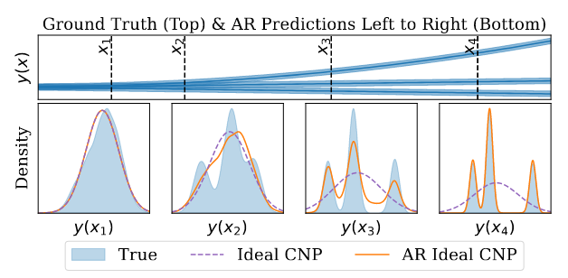
图 3：顶部：生成过程：三个确定性函数与加性高斯噪声的混合模型。底部：在虚线指示的四个目标位置，窗格从左到右显示了理想条件神经过程的真实分布和预测，以及应用了自回归的理想条件神经过程。见附录 D.3 和 E。

（4）一致性和自回归设计空间

如 表(1) 所示，自回归条件神经过程放弃了一致性的基本性质，因为分布 $\{\mathrm{AR}_{\mathbf{x}}(\pi_{\theta}, D^{(c)}_m) : \mathbf{x} \in \mathcal{X}^N, N \in \mathbb{N}\}$ 在重排或边缘化时存在不一致：重排 $\mathbf{x}$ 和边缘化目标点会改变分布。这违背了 Kolmogorov 定理（Oksendal，2013 年）的条件，阻止了定义一致性随机过程的分布。因此，在使用自回归条件神经过程时涉及很大的设计空间，其中原本对其他的神经过程预测没有影响的一些场景，现在有可能显著影响我们的性能。

其中一种选择是： 一次采样多少点 。一次仅采样一个点会导致所有点之间的依赖关系，但需要做 $N$ 次前向传递。或者，我们可以将 $x^{(t)}$ 中的 $N$ 个输入分成由 $K$ 个点组成的块，并对每个块使用单次条件神经过程前向传递进行采样。这需要 $N/K$ 次前向传递，不过同一块中的点之间条件独立。当 $K = N$ 时就对应标准的条件神经过程预测；如果 $K = 1$ ，则恢复 程序 2.1。这为从业者提供了一个选择，可以在 “更快、一致但表现力较低的标准条件神经过程预测” 和 “更慢、不太一致但更具表现力的自回归预测” 之间进行权衡。在本文中，我们使用 $K = 1$ 的全自回归模式，并将块自回归采样的调查留给未来的工作。

（5）获得平滑的样本

由于自回归模式缺乏一致性，目标点之间的间距选择会显著影响性能。例如，必须注意目标点的数量不要比训练期间看到的环境点数量大很多，以避免在测试时，模型面临分布外背景集的大小。这就提出了如何在非常精细的网格上对函数进行采样的问题。此外， 由于条件神经过程不区分 认知不确定性 和 任意不确定性 ，因此不清楚如何获得平滑、无噪声的样本，（平滑无噪声样本指 $f$ 未被 式 (4) 中的 i.i.d. 噪声 $\varepsilon$ 破坏的那些样本）。以下命题表明，对于被加性噪声破坏的平滑样本，平滑分量可以用以噪声观测为条件的预测均值来近似：

【命题 2.2（平滑样本的恢复）】

设 $\mathcal{X} \subseteq \mathbb{R}$ 是紧致的，设 $f$ 是一个具有连续样本路径且 $\mathrm{sup}_{x \in \mathcal{X}} \|f(x)\|_{L^2} < \infty$ 的随机过程。设 $(\varepsilon_n)_{n \geq 0}$ 为独立同分布的随机变量（可能非高斯），使得 $\mathbb{E}[\varepsilon_0] = 0$ 且 $\mathbb{V}[\varepsilon_0] < \infty$。考虑任意序列 $(x_n)_{n \geq 1} \subseteq \mathcal{X}$ ，设 $x^* \in \mathcal{X}$ 为 $(x_n)_{n \geq 1}$ 的极限点。如果 $y(x^*) = f(x^*) + \varepsilon_0$ 和 $y_n = f (x_n) + \varepsilon_n$ 是 $f$ 的含噪声观测，则几乎可以肯定：

$$\lim_{n \rightarrow \infty} \mathbb{E}[y(x^*) | y_1,\ldots , y_n] = f(x^*) \tag{8}$$

我们在 附录 B 中提供了证明。式 (8) 提示我们使用以下两步过程在自回归条件神经过程中获取平滑样本：

• 第 1 步：令 $\mathbf{x}_{1:n}$ 为不超过训练期间看到的点数的多个目标输入。采样得到 $\mathbf{y}_{1:n} \sim \mathrm{AR}_{\mathbf{x}_{1:n}}(\pi_{\theta}, D^{(c)}_m)$ ，该样本包括观测噪声。
• 第 2 步：通过再次让样本通过模型来去除样本中的噪声： $\mathcal{N}(\boldsymbol{\mu}_{1:n}, \mathbf{D}) = P_{\mathbf{x}_{1:n}} \pi_{\theta}(D^{(c)}_m \oplus (\mathbf{x}_{1:n}, \mathbf{y}_{1:n}))$ 。这里预测均值 $\boldsymbol{\mu}_{1:n}$ 形成无噪声样本。要在任意多个输入下生成样本，还可以计算 $N(\boldsymbol{\mu}'_{1:n}, \mathbf{D}) = P_{\mathbf{x}'_{1:n}} \pi_{\theta}(D^{(c)}_m \oplus (\mathbf{x}_{1:n}, \mathbf{y}_{1:n}))$ 其中 $\mathbf{x}'_{1:n}$ 是任意的。此过程的结果如图 4 所示，并用于生成图 1（右）所示的无噪声样本。附录 C 中的图 7 也以图形方式逐步说明了这个两步过程。

图 4：比较来自自回归ConvCNP 的无噪声（蓝色）和有噪声（红色）样本。采用了两套样本数据，分别来自具有指数二次核的高斯过程采样数据，以及地面真实的高斯过程。无噪声自回归样本是使用命题 2.2 建议的程序从噪声自回归样本生成的。

3 与其他神经分布估计的关系

已经为 神经分布估计 (NDE) 开发了各种模型：

• 归一化流（Dinh 等，2015 年 ^[21]）
• 生成对抗网络（GANs；Goodfellow 等，2014 年 ^[32]）
• 变分自编码器（VAEs；Kingma & Welling，2014 年 ^[48]）
• 自回归模型（Uria 等，2016 年 ^[85]）
• 扩散模型（Sohl-Dickstein 等，2015 年^[80]；Ho 等，2020 年^[40]）。

图 5 可视化了 神经分布估计模型 的概况。我们认为神经过程和自回归条件神经过程应被视为一种神经分布估计器 (NDE)，并应当纳入该一览图中。

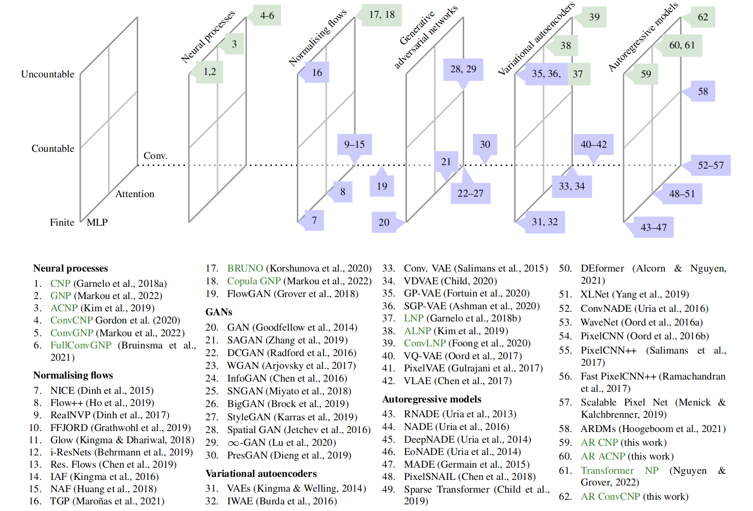
图 5：展示了 AR条件神经过程与各种神经分布估计器之间关系的概念图。垂直轴表示模型是学习有限数量随机变量、可数无限数还是不可数无限数的分布。指向页内的轴表示该架构是基于 MLP，还是使用注意力或卷积。从左到右，展示了不同的建模范例。当神经过程（以绿色突出显示）被引入其他建模范例时，就会发生富有成效的交流。我们提出的 AR条件神经过程可以看作是将神经过程引入自回归建模范例。

（1）自回归条件神经过程与传统自回归模型

自回归条件神经过程继承了自回归模型的优势，例如以易于处理的似然对复杂依赖关系进行建模，但也继承了其弱点，最明显的是测试时间的采样速度慢。采样速度慢是自回归条件神经过程的主要缺点，尽管可以采用加速自回归模型的一些技术（Ramachandran 等，2017 年^[74]）。

自回归条件神经过程与现有自回归模型之间的一个主要区别是： 自回归条件神经过程分解了不可数无限变量集的联合分布，允许在任意输入位置处进行查询。

与 DEformer (Alcorn & Nguyen, 2021 ^[1])、EoNADE (Uria 等, 2014 ^[84]) 和 XLnet (Yang 等, 2019 ^[91]) 一样，自回归条件神经过程被训练为不特定于将联合分布分解为任何指定顺序的条件分布。为了实现这一目标，自回归条件神经过程与其他自回归模型共享了如下设计选择：

• 共享用于生成每个条件分布的架构，类似于 WaveNet（Oord 等，2016a ^[70]）和 PixelCNN（Oord 等，2016b ^[71]）);
• 数据点索引作为 DEformer 模型中神经网络的输入（Alcorn & Nguyen，2021 ^[1]）；
• 训练最大化对数似然，包括联合分布的所有组分，类似于 EoNADE（Uria 等，2014 年 ^[84] ）和 XLnet（Yang 等，2019 年 ^[91]）。

（2）神经过程与变分自编码器、归一化流

图 5 还显示了神经过程、变分自编码器、归一化流之间的联系。

• 与变分自编码器一样，隐神经过程使用解码器对分解后组分的分布进行参数化，并依靠隐变量来归纳依赖性。关键区别在于隐神经过程对不可数变量集的分布进行了建模。
• 条件 BRUNO（Korshunova 等，2020 年 ^[51]）和 copula GNPs（Markou 等，2022 年 ^[61]）等模型结合了神经过程和归一化流的思想，将随机过程转换为一种可逆转换。
• 诸如 Spatial GAN (Jetchev 等, 2016 ^[undefined]) 和 $\infty$ -GAN (Lu 等, 2020 ^[54]) 等 GAN 模型对可数变量进行了建模，例如任意大小的图像。检查 图 5，我们看到 GAN 是描述的唯一一类当前没有神经过程版本（即一个对无数变量建模的版本）的模型。这表明神经过程的对抗训练是未来研究的一个有趣方向。

在最近的工作中，Nguyen & Grover (2022) 提出了 Transformer 神经过程 (TNPs)，它使用具有自回归似然的 causally-masked transformer 架构。相比之下，我们的工作重点不是提出新的自回归架构，而是在自回归模式下运行现有的条件神经过程以获得具有相干性的样本和改进的似然，而无需修改架构或训练程序。

在之前的工作中，Volpp 等(2021 ^[89]) 使用自回归采样来可视化来自条件神经过程的样本。不过，其工作重点在于为神经过程提出一种新的环境聚合机制，并且它们没有自回归地计算条件神经过程的似然，也没有研究任何性能提升。

4 自回归神经过程的性能

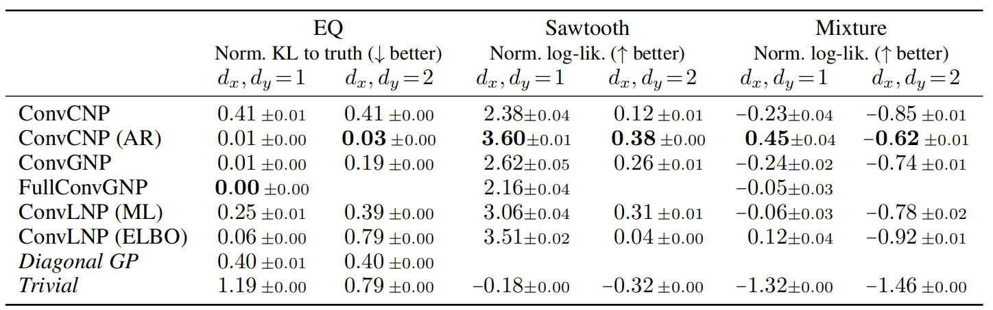
表 2：神经过程在 GP EQ 任务、锯齿波任务和混合任务上的训练表现。对角线 GP 表示精确的 GP 预测，但删除了相关性。 Trivial 表示一个模型，该模型使用上下文输出的经验均值和标准差来预测高斯分布。明显最好的模型以粗体显示。请注意，全卷积神经过程不能在 dx > 1 的任务上运行。

表 3：捕食者-猎物实验中的归一化对数似然，显示模拟 (S) 和真实 ® 数据的插值 (int.)、预测 (for.) 和重建 (rec.)。显着最好的结果以粗体表示。

表 4：脑电图实验的标准化对数似然。显着最好的结果以粗体表示。

表 5：2019-2019 年云覆盖任务测试期间的归一化对数似然和平均绝对误差（MAE，以云覆盖百分比为单位）。请注意，不能直接比较高斯和 beta 分类模型的对数似然。错误表示标准错误。显着最好的结果以粗体表示。

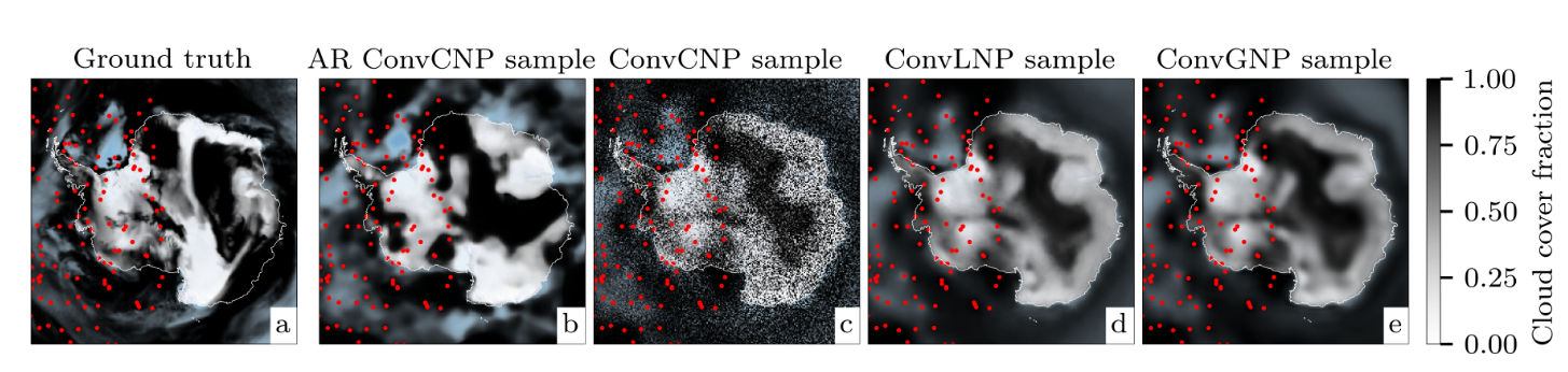
图 6：(a) Ground truth 模拟了 2018 年 6 月 25 日的云层覆盖率。 (b-e)，样本来自自回归ConvCNP、ConvCNP、ConvLNP 和 ConvGNP，上下文点用红点表示。从 2D 空间的右侧移除了上下文点，以测试模型推断远离观测点的相干函数样本的能力。 ConvCNP 和 ConvLNP 模型使用 beta 分类似然，而 ConvGNP 使用低秩高斯似然。

表 6：降尺度实验中的归一化对数似然和平均绝对误差 (MAE)，没有（左）和有（右）辅助气象站观测。显着最好的结果以粗体表示。 ∗不能使用额外的气象站观测。

4 自回归神经过程的表现

4.1 合成生成的高斯和非高斯数据

4.2 使用 LOTKA-VOLTERRA 方程从 SIM 到真实的传输

4.3 脑电图实验

4.4 环境建模

5 局限性和结论

我们已经表明，AR 程序可以很容易地应用于提高条件神经过程的性能，产生连贯样本并显著提高似然。令人惊讶的是，在广泛的实验中，这种简单方法通常优于依赖隐变量或明确建模相关性的更复杂的方法。我们通过将自回归条件神经过程应用于气候数据融合任务、对 $[0, 1]$ 约束数据进行建模并引入一种新的多尺度架构，证明了我们的方法对现实世界感兴趣的数据集的有效性。

值得注意的是，自回归条件神经过程通过启用联合非高斯预测填补了气候建模工具箱中的空白，这可用于更好地估计复合风险的大小。我们还将自回归条件神经过程置于更大的神经密度估计范畴中，展示了将神经过程与其他建模范例相结合的成果。

更一般地说，自回归条件神经过程为神经过程框架配备了一个新的选择，在此选项中，训练时的建模复杂性和计算开销可以与测试时的计算开销进行权衡。特别是，通过自回归应用神经过程获得的更高质量的样本和更好的似然伴随着对目标集中的每个元素执行前向传递的额外成本。这对于大型目标集来说可能非常昂贵，并且构成了使用自回归条件神经过程的主要实际缺陷。

此外，由于自回归条件神经过程没有定义一致性的随机过程，因此自回归过程的设计选择可能会影响结果的质量。因此，从业者需要避免选择导致病态行为的目标集，例如当目标输入的空间密度过高时。但这种设计空间的灵活性也带来了机会：例如，在 附录 M 中，我们展示了可以使用辅助目标点来进一步改进预测。

最后，未来工作的有前途的途径包括将自回归程序应用于除条件神经过程之外的其他神经过程，以及研究 第 2 节 中介绍的块抽样方案的有效性。

6 再现性声明

我们所有的实验都是使用合成或公开可用的数据集进行的。 EEG 数据集可通过 UCI 数据库获得，环境数据也可通过欧洲气候数据服务公开获得

我们公开了所有必要的代码来重现实验以及下载、预处理和模拟南极云层数据的说明。 命题 2.1 和 命题 2.2 的证明分别在 附录 A 和 附录 B 中给出。有关模型架构和实验设置的详细信息，请参见合成数据集的 附录 F 至 附录 H 、模拟到真实传输实验的 附录 I 、EEG 实验的 附录 J 、数据同化实验的 附录 K ，以及 附录 L 为降尺度实验。

7 道德声明

训练条件神经过程可以自回归地显著提高它们的表现，但我们预计本文工作不会产生不利的社会影响。话虽如此，捕获数据集中存在的统计趋势的问题必须小心执行，尤其是在安全关键应用程序中，在这些应用程序中做出不正确和自信的预测可能会产生严重后果。我们将自回归程序视为捕获此类行为的有用工具，而不是灵丹妙药，并希望本文工作能够鼓励进一步研究为此建立有效但可靠的模型。

我们还注意到，虽然训练条件神经过程在计算上比替代神经过程模型更便宜，但自回归采样本身会在测试时产生大量计算成本，从而产生能源成本。大规模运行自回归采样可能会导致对这些模型的功率需求更大，从而导致更大的碳足迹，这是不可取的。然而，我们认为环境建模的潜在好处可能超过此成本，而利用方法使自回归条件神经过程的计算效率更高应该有助于缓解这个问题。

参考文献

• [1] Michael A. Alcorn, Anh Nguyen. The DEformer: An order-agnostic distribution estimating transformer. ICML Workshop on Invertible Neural Networks, Normalizing Flows, and Explicit Likelihood Models (INNF+), 2021.
• [2] Martin Arjovsky, Soumith Chintala, and Leon Bottou. Wasserstein generative adversarial networks. In Proceedings of the 34th International Conference on Machine Learning, volume 70 of Proceedings of Machine Learning Research, pp. 214–223.PMLR, 2017.
• [3] Matthew Ashman, Jonathan So, Will Tebbutt, Vincent Fortuin, Michael Pearce, and Richard E. Turner. Sparse Gaussian process variational autoencoders. arXiv preprint arXiv:2010.10177, 2020.
• [4] Jimmy Lei Ba, Jamie Ryan Kiros, and Geoffrey E. Hinton. Layer normalization. Neural Information Processing Systems Deep Learning Symposium, 2016.
• [5] Henri Begleiter. EEG database data set, 2022.
• [6] Jens Behrmann, Will Grathwohl, Ricky T. Q. Chen, David Duvenaud, and Jörn-Henrik Jacobsen. Invertible residual networks. In Proceedings of 36th International Conference on Machine Learning, volume 97 of Proceedings of Machine Learning Research.PMLR, 2019.
• [7] Andrew Brock, Jeff Donahue, and Karen Simonyan. Large scale GAN training for high fidelity natural image synthesis. In Proceedings of the 7th International Conference on Learning Representations, 2019.
• [8] Wessel P. Bruinsma, James Requeima, Andrew Y. K. Foong, Jonathan Gordon, and Richard E. Turner. The Gaussian neural process. In Proceedings of the 3rd Symposium on Advances in Approximate Bayesian Inference, 2021.
• [9] Y. Burda, R. Grosse, and R. Salakhutdinov. Importance weighted autoencoders. In Advances in Neural Information Processing Systems 29. Curran Associates, Inc., 2016.
• [10] Ni-Bin Chang, Kaixu Bai. Multisensor data fusion and machine learning for environmental remote sensing. CRC Press, 2018.
• [11] Ricky T. Q. Chen, Jens Behrmann, David K. Duvenaud, and Jörn-Henrik Jacobsen. Residual flows for invertible generative modeling. Advances in Neural Information Processing Systems, 32, 2019.
• [12] X. Chen, Y. Duan, R. Houthooft, J. Schulman, I. Sutskever, and P. Abbeel. InfoGAN: Interpretable representation learning by information maximizing generative adversarial nets. In Advances in Neural Information Processing Systems 29. Curran Associates, Inc., 2016.
• [13] X. Chen, D. P. Kingma, T. Salimans, Y. Duan, P. Dhariwal, J. Schulman, I. Sutskever, and P. Abbeel. Variational lossy autoencoder. In Proceedings of the 5th International Conference on Learning Representations, 2017.
• [14] Xi Chen, Nikhil Mishra, Mostafa Rohaninejad, and Pieter Abbeel. PixelSNAIL: An improved autoregressive generative model. In International Conference on Machine Learning, pp. 864–872.PMLR, 2018.
• [15] Rewon Child. Very deep VAEs generalize autoregressive models and can outperform them on images. In Proceedings of the 9th International Conference on Learning Representations2020] Rewon Child. Very deep VAEs generalize autoregressive models and can outperform them on images. In Proceedings of the 9th International Conference on Learning Representations, 2020.
• [16] Rewon Child, Scott Gray, Alec Radford, and Ilya Sutskever. Generating long sequences with sparse transformers. arXiv preprint arXiv:1904.10509, 2019.
• [17] Franccois Chollet. Xception: Deep learning with depthwise separable convolutions. In Proceedings of the IEEE/CVF Conference on Computer Vision and Pattern Recognition, 2017.
• [18] D. P. Dee, S. M. Uppala, A. J. Simmons, P. Berrisford, P. Poli, S. Kobayashi, U. Andrae, M. A. Balmaseda, G. Balsamo, P. Bauer, P. Bechtold, A. C. M. Beljaars, L. van de Berg, J. Bidlot, N. Bormann, C. Delsol, R. Dragani, M. Fuentes, A. J. Geer, L. Haimberger, S. B. Healy, H. Hersbach, E. V. Holm, L. Isaksen, P. Kållberg, M. Kohler, M. Matricardi, A. P. McNally, B. M. Monge-Sanz, J.-J. Morcrette, B.-K. Park, C. Peubey, P. de Rosnay, C. Tavolato, J.-N. Thepaut, and F. Vitart. The ERA-interim reanalysis: Configuration and performance of the data assimilation system. Quarterly Journal of the Royal Meteorological Society, 137(656):553–597, 2011.
• [19] Adji B Dieng, Francisco JR Ruiz, David M Blei, and Michalis K Titsias. Prescribed generative adversarial networks. arXiv preprint arXiv:1910.04302, 2019.
• [20] L. Dinh, J. Sohl-Dickstein, and S. Bengio. Density estimation using real NVP. In Proceedings of the 5th International Conference on Learning Representations, 2017.
• [21] Laurent Dinh, David Krueger, and Yoshua Bengio. NICE: Non-linear independent components estimation. In International Conference on Learning Representations, 2015.
• [22] Richard Durrett. Probability: Theory and Examples. Cambridge University Press, 4 edition, 2010.
• [23] Earth Resources Observation and Science Center, U.S. Geological Survey, U.S. Department of the Interior. USGS 30 arc-second global elevation data, GTOPO30, 1997.
• [24] Pau Ferrer-Cid, Jose M Barcelo-Ordinas, Jorge Garcia-Vidal, Anna Ripoll, and Mar Viana. Multisensor data fusion calibration in IoT air pollution platforms. IEEE Internet of Things Journal, 7(4): 3124–3132, 2020.
• [25] Andrew Y. K. Foong, Wessel P. Bruinsma, Jonathan Gordon, Yann Dubois, James Requeima, and Richard E. Turner. Meta-learning stationary stochastic process prediction with convolutional neural processes. In Advances in Neural Information Processing Systems 33. Curran Associates, Inc., 2020.
• [26] Vincent Fortuin, Dmitry Baranchuk, Gunnar Rätsch, and Stephan Mandt. GP-VAE: Deep probabilistic time series imputation. In International conference on artificial intelligence and statistics, pp. 1651–1661.PMLR, 2020.
• [27] M. Garnelo, D. Rosenbaum, C. J. Maddison, T. Ramalho, D. Saxton, M. Shanahan, Y. Whye Teh, D. J. Rezende, and S. M. A. Eslami. Conditional neural processes. In Proceedings of 35th International Conference on Machine Learning, volume 80 of Proceedings of Machine Learning Research.PMLR, 2018a.
• [28] M. Garnelo, J. Schwarz, D. Rosenbaum, F. Viola, D. J. Rezende, S. M. A. Eslami, and Y. Whye Teh. Neural processes. In Theoretical Foundations and Applications of Deep Generative Models Workshop, 35th International Conference on Machine Learning, 2018b.
• [29] A. J. Geer. Learning earth system models from observations: machine learning or data assimilation? Philosophical Transactions of the Royal Society A: Mathematical, Physical and Engineering Sciences, 379(2194):20200089, February 2021.
• [30] Mathieu Germain, Karol Gregor, Iain Murray, and Hugo Larochelle. MADE: Masked autoencoder for distribution estimation. In International conference on machine learning, pp. 881–889.PMLR, 2015.
• [31] Andrew Gettelman, Alan J Geer, Richard M Forbes, Greg R Carmichael, Graham Feingold, Derek J Posselt, Graeme L Stephens, Susan C van den Heever, Adam C Varble, and Paquita Zuidema. The future of earth system prediction: Advances in model-data fusion. Science Advances, 8(14): eabn3488, 2022.
• [32] I. J. Goodfellow, J. Pouget Abadie, M. Mirza, B. Xu, D. Warde Farley, S. Ozair, A. Courville, and Y. Bengio. Generative adversarial networks. In Advances in Neural Information Processing Systems 27, volume 27. Curran Associates, Inc., 2014.
• [33] Jonathan Gordon, Wessel P. Bruinsma, Andrew Y. K. Foong, James Requeima, Yann Dubois, and Richard E. Turner. Convolutional conditional neural processes. In Proceedings of the 8th International Conference on Learning Representations, 2020.
• [34] Will Grathwohl, Ricky T. Q. Chen, Jesse Bettencourt, Ilya Sutskever, and David Duvenaud. FFJORD: Free-form continuous dynamics for scalable reversible generative models. In Proceedings of the 7th International Conference on Learning Representations, 2019.
• [35] Aditya Grover, Manik Dhar, and Stefano Ermon. Flow-GAN: Combining maximum likelihood and adversarial learning in generative models. In Proceedings of the AAAI Conference on Artificial Intelligence, volume 32, 2018.
• [36] Ishaan Gulrajani, Kundan Kumar, Faruk Ahmed, Adrien Ali Taiga, Francesco Visin, David Vazquez, and Aaron Courville. PixelVAE: A latent variable model for natural images. In Proceedings of the 5th International Conference on Learning Representations, 2017.
• [37] Kaiming He, Xiangyu Zhang, Shaoqing Ren, and Jian Sun. Deep residual learning for image recognition. In Proceedings of the IEEE/CVF Conference on Computer Vision and Pattern Recognition, 2016.
• [38] Hans Hersbach, Bill Bell, Paul Berrisford, Shoji Hirahara, András Horányi, Joaquín Muñoz-Sabater, Julien Nicolas, Carole Peubey, Raluca Radu, Dinand Schepers, Adrian Simmons, Cornel Soci, Saleh Abdalla, Xavier Abellan, Gianpaolo Balsamo, Peter Bechtold, Gionata Biavati, Jean Bidlot, Massimo Bonavita, Giovanna De Chiara, Per Dahlgren, Dick Dee, Michail Diamantakis, Rossana Dragani, Johannes Flemming, Richard Forbes, Manuel Fuentes, Alan Geer, Leo Haimberger, Sean Healy, Robin J. Hogan, Elias Holm, Marta Janiskova, Sarah Keeley, Patrick Laloyaux, Philippe Lopez, Cristina Lupu, Gabor Radnoti, Patricia de Rosnay, Iryna Rozum, Freja Vamborg, Sebastien Villaume, and Jean-Noël Thépaut. The ERA5 global reanalysis. 146(730):1999–2049, 2020.
• [39] Jonathan Ho, Xi Chen, Aravind Srinivas, Yan Duan, and Pieter Abbeel. Flow++: Improving flowbased generative models with variational dequantization and architecture design. In International Conference on Machine Learning, pp. 2722–2730.PMLR, 2019.
• [40] Jonathan Ho, Ajay Jain, and Pieter Abbeel. Denoising diffusion probabilistic models. Advances in Neural Information Processing Systems, 33:6840–6851, 2020.
• [41] Emiel Hoogeboom, Alexey A Gritsenko, Jasmijn Bastings, Ben Poole, Rianne van den Berg, and Tim Salimans. Autoregressive diffusion models. In Proceedings of the 10th International Conference on Learning Representations, 2021.
• [42] Marjan Hosseini and Reza Kerachian. A data fusion-based methodology for optimal redesign of groundwater monitoring networks. Journal of Hydrology, 552:267–282, 2017.
• [43] Chin-Wei Huang, David Krueger, Alexandre Lacoste, and Aaron Courville. Neural autoregressive flows. In International Conference on Machine Learning, pp. 2078–2087.PMLR, 2018.
• [44] Douglas R. Hundley. Introduction to mathematical modelling. URL http://people.whitman. edu/~hundledr/courses/M250F03/M250.html. Nikolay Jetchev, Urs Bergmann, and Roland Vollgraf. Texture synthesis with spatial generative adversarial networks. In Workshop on Adversarial Training of Advances, Neural Information Processing Systems 29, 2016.
• [45] Tero Karras, Samuli Laine, and Timo Aila. A style-based generator architecture for generative adversarial networks. In Proceedings of the IEEE/CVF conference on computer vision and pattern recognition, pp. 4401–4410, 2019.
• [46] H. Kim, A. Mnih, J. Schwarz, M. Garnelo, A. Eslami, D. Rosenbaum, O. Vinyals, and Y. Whye Teh. Attentive neural processes. In Proceedings of the 7th International Conference on Learning Representations, 2019.
• [47] D. P. Kingma and J. Ba. ADAM: A method for stochastic optimization. In Proceedings of the 3rd International Conference on Learning Representations, 2015.
• [48] D. P. Kingma and M. Welling. Auto-encoding variational Bayes. In Proceedings of the 2rd International Conference on Learning Representations, 2014.
• [49] D. P. Kingma, T. Salimans, R. Jozefowicz, X. Chen, I. Sutskever, and M. Welling. Improving variational inference with inverse autoregressive flow. In Advances in Neural Information Processing Systems 29. Curran Associates, Inc., 2016.
• [50] Durk P Kingma and Prafulla Dhariwal. Glow: Generative flow with invertible 1x1 convolutions. Advances in neural information processing systems, 31, 2018.
• [51] Iryna Korshunova, Yarin Gal, Arthur Gretton, and Joni Dambre. Conditional BRUNO: A neural process for exchangeable labelled data. Neurocomputing, 416:305–309, 2020.
• [52] Dana Lahat, Tülay Adali, and Christian Jutten. Multimodal data fusion: An overview of methods, challenges, and prospects. Proceedings of the IEEE, 103(9):1449–1477, 2015.
• [53] Alfred J. Lotka. Contribution to the theory of periodic reactions. The Journal of Physical Chemistry, 14(3):271–274, 1910.
• [54] Chaochao Lu, Richard E. Turner, Yingzhen Li, and Nate Kushman. Interpreting spatially infinite generative models. In ICML Workshop on Human Interpretability in Machine Learning, 2020.
• [55] Zhenyu Lu, Jungho Im, Lindi Quackenbush, and Kerry Halligan. Population estimation based on multi-sensor data fusion. International Journal of Remote Sensing, 31(21):5587–5604, 2010.
• [56] D. A. MacLulich. Fluctuations in the Numbers of the Varying Hare (Lepus Americanus). University of Toronto Press, 1937.
• [57] Douglas Maraun and Martin Widmann. Statistical Downscaling and Bias Correction for Climate Research. Cambridge Uiversity Press, 2018.
• [58] Douglas Maraun, Martin Widmann, José M. Gutiérrez, Sven Kotlarski, Richard E. Chandler, Elke Hertig, Joanna Wibig, Radan Huth, and Renate A. I. Wilcke. VALUE: A framework to validate downscaling approaches for climate change studies. Earth’s Future, 3(1):1–14, 2015.
• [59] Douglas Maraun, Theodore G. Shepherd, Martin Widmann, Giuseppe Zappa, Daniel Walton, José M. Gutiérrez, Stefan Hagemann, Ingo Richter, Pedro M. M. Soares, Alex Hall, and Linda O. Mearns. Towards process-informed bias correction of climate change simulations. Nature Climate Change, 7(11):764–773, 2017.
• [60] Stratis Markou, James Requeima, Wessel P. Bruinsma, and Richard E. Turner. Efficient Gaussian neural processes for regression. In Workshop on Uncertainty & Robustness in Deep Learning, 39th International Conference on Machine Learning, 2021.
• [61] Stratis Markou, James Requeima, Wessel P. Bruinsma, Anna Vaughan, and Richard E. Turner. Practical conditional neural processes via tractable dependent predictions. In Proceedings of the 10th International Conference on Learning Representations, 2022.
• [62] Juan Maroñas, Oliver Hamelijnck, Jeremias Knoblauch, and Theodoros Damoulas. Transforming gaussian processes with normalizing flows. In International Conference on Artificial Intelligence and Statistics, pp. 1081–1089.PMLR, 2021.
• [63] Jacob Menick and Nal Kalchbrenner. Generating high fidelity images with subscale pixel networks and multidimensional upscaling. In Proceedings of the 7th International Conference on Learning Representations, 2019.
• [64] Thomas P. Minka. Expectation propagation for approximate Bayesian inference. In Conference in Uncertainty in Artificial Intelligence, volume 17, pp. 362–369. Morgan Kaufmann Publishers Inc., 2001.
• [65] Takeru Miyato, Toshiki Kataoka, Masanori Koyama, and Yuichi Yoshida. Spectral normalization for generative adversarial networks. In Proceedings of the 6th International Conference on Learning Representations, 2018.
• [66] M. Morlighem. Measures bedmachine antarctica, version 2, 2020.
• [67] Tung Nguyen and Aditya Grover. Transformer neural processes: Uncertainty-aware meta learning via sequence modeling. In International Conference on Machine Learning, pp. 16569–16594.PMLR, 2022.
• [68] Augustus Odena, Vincent Dumoulin, and Chris Olah. Deconvolution and Checkerboard Artifacts. Distill, 1(10):e3, October 2016.
• [69] Bernt Oksendal. Stochastic differential equations: an introduction with applications. Springer Science & Business Media, 2013.
• [70] Aaron van den Oord, Sander Dieleman, Heiga Zen, Karen Simonyan, Oriol Vinyals, Alex Graves, Nal Kalchbrenner, Andrew Senior, and Koray Kavukcuoglu. WaveNet: A generative model for raw audio. arXiv preprint arXiv:1609.03499, 2016a.
• [71] Aaron van den Oord, Nal Kalchbrenner, Lasse Espeholt, Oriol Vinyals, Alex Graves, 等 Conditional image generation with PixelCNN decoders. Advances in neural information processing systems, 29, 2016b.
• [72] Aaron van den Oord, Oriol Vinyals, 等 Neural discrete representation learning. Advances in neural information processing systems, 30, 2017.
• [73] Alec Radford, Luke Metz, and Soumith Chintala. Unsupervised representation learning with deep convolutional generative adversarial networks. In Unsupervised Representation Learning with Deep Convolutional Generative Adversarial Networks, 2016.
• [74] Prajit Ramachandran, Tom Le Paine, Pooya Khorrami, Mohammad Babaeizadeh, Shiyu Chang, Yang Zhang, Mark A. Hasegawa-Johnson, Roy H. Campbell, and Thomas S. Huang. Fast generation for convolutional autoregressive models. In Workshop Track, International Conference on Learning Representations, 2017.
• [75] Suman Ravuri, Karel Lenc, Matthew Willson, Dmitry Kangin, Remi Lam, Piotr Mirowski, Megan Fitzsimons, Maria Athanassiadou, Sheleem Kashem, Sam Madge, Rachel Prudden, Amol Mandhane, Aidan Clark, Andrew Brock, Karen Simonyan, Raia Hadsell, Niall Robinson, Ellen Clancy, Alberto Arribas, and Shakir Mohamed. Skilful precipitation nowcasting using deep generative models of radar. Nature, 597(7878):672–677, September 2021.
• [76] Caleb Robinson, Kolya Malkin, Nebojsa Jojic, Huijun Chen, Rongjun Qin, Changlin Xiao, Michael Schmitt, Pedram Ghamisi, Ronny Hänsch, and Naoto Yokoya. Global land-cover mapping with weak supervision: Outcome of the 2020 IEEE GRSS data fusion contest. IEEE Journal of Selected Topics in Applied Earth Observations and Remote Sensing, 14:3185–3199, 2021.
• [77] Olaf Ronneberger, Philipp Fischer, and Thomas Brox. U-Net: Convolutional networks for biomedical image segmentation. In International Conference on Medical image computing and computerassisted intervention, pp. 234–241. Springer, 2015.
• [78] Tim Salimans, Diederik Kingma, and Max Welling. Markov chain Monte Carlo and variational inference: Bridging the gap. In International Conference on Machine Learning, pp. 1218–1226.PMLR, 2015.
• [79] Tim Salimans, Andrej Karpathy, Xi Chen, and Diederik P Kingma. PixelCNN++: Improving the PixelCNN with discretized logistic mixture likelihood and other modifications. arXiv preprint arXiv:1701.05517, 2017.
• [80] Jascha Sohl-Dickstein, Eric Weiss, Niru Maheswaranathan, and Surya Ganguli. Deep unsupervised learning using nonequilibrium thermodynamics. In International Conference on Machine Learning, pp. 2256–2265.PMLR, 2015.
• [81] Thomas F. Stocker, Dahe Qin, Gian-Kasper Plattner, Melinda M.B. Tignor, Simon K. Allen, Judith Boschung, Alexander Nauels, Yu Xia, Vincent Bex, and Pauline M. Midgley. Climate change 2013: The physical science basis. Technical report, Cambridge University Press, 2013.
• [82] A. M. G. Klein Tank, J. B. Wijngaard, G. P. Können, R. Böhm, G. Demarée, A. Gocheva, M. Mileta, S. Pashiardis, L. Hejkrlik, C. Kern-Hansen, R. Heino, P. Bessemoulin, G. Müller-Westermeier, M. Tzanakou, S. Szalai, T. Pálsdóttir, D. Fitzgerald, S. Rubin, M. Capaldo, M. Maugeri, A. Leitass, A. Bukantis, R. Aberfeld, A. F. V. van Engelen, E. Forland, M. Mietus, F. Coelho, C. Mares, V. Razuvaev, E. Nieplova, T. Cegnar, J. Antonio López, B. Dahlström, A. Moberg, W. Kirchhofer, A. Ceylan, O. Pachaliuk, L. V. Alexander, and P. Petrovic. Daily dataset of 20thcentury surface air temperature and precipitation series for the european climate assessment. International Journal of Climatology, 22(12):1441–1453, 2002.
• [83] Benigno Uria, Iain Murray, and Hugo Larochelle. RNADE: The real-valued neural autoregressive density-estimator. Advances in Neural Information Processing Systems, 26, 2013.
• [84] Benigno Uria, Iain Murray, and Hugo Larochelle. A deep and tractable density estimator. In International Conference on Machine Learning, pp. 467–475.PMLR, 2014.
• [85] Benigno Uria, Marc-Alexandre Côté, Karol Gregor, Iain Murray, and Hugo Larochelle. Neural autoregressive distribution estimation. Journal of Machine Learning Research, 17(205):1–37, 2016.
• [86] A. Vaswani, N. Shazeer, N. Parmar, J. Uszkoreit, L. Jones, A. N. Gomez, L. Kaiser, and I. Polosukhin. Attention is all you need. In Advances in Neural Information Processing Systems 30. Curran Associates, Inc., 2017.
• [87] A. Vaughan, W. Tebbutt, J. S. Hosking, and R. E. Turner. Convolutional conditional neural processes for local climate downscaling. Geoscientific Model Development, 15(1):251–268, 2022.
• [88] Oriol Vinyals, Charles Blundell, Timothy Lillicrap, Koray Kavukcuoglu, and Daan Wierstra. Matching networks for one shot learning. In Advances in Neural Information Processing Systems 29. Curran Associates, Inc., 2016.
• [89] Michael Volpp, Fabian Flürenbrock, Lukas Grossberger, Christian Daniel, and Gerhard Neumann. Bayesian context aggregation for neural processes. In International Conference on Learning Representations, 2021.
• [90] V. Volterra. Variazioni e fluttuazioni del bumero d’ondividui in specie animali conviventi. Memoria della Reale Accademia Nazionale dei Lincei, 2:31–113, 1926.
• [91] Zhilin Yang, Zihang Dai, Yiming Yang, Jaime Carbonell, Russ R Salakhutdinov, and Quoc V Le. XLNet: Generalized autoregressive pretraining for language understanding. Advances in neural information processing systems, 32, 2019.
• [92] Han Zhang, Ian Goodfellow, Dimitris Metaxas, and Augustus Odena. Self-attention generative adversarial networks. In International conference on machine learning, pp. 7354–7363.PMLR, 2019.
• [93] X. L. Zhang, H. Begleiter, B. Porjesz, W. Wang, and A. Litke. Event related potentials during object recognition tasks. Brain Research Bulletin, 38(6):531–538, 1995.