第三章：线性模型与概率编程语言¶

随着概率编程语言的出现，现代贝叶斯建模只需要编码一个模型和 “按一个按钮 “那样简单。然而，有效模型的建立和分析通常需要更多的工作。

随着本书的推进，我们将建立许多不同类型的模型，但在本章中将从最简单的线性模型开始。线性模型是一类广泛应用的模型，其中一个指定观测值（结果变量）的期望值是相关预测因子（预测变量）的线性组合。

深刻理解拟合和解释线性模型的方法，是后续很多模型的坚实基础；并将有助于我们巩固『贝叶斯推断（第 1 章）』和『贝叶斯模型的探索性分析（第 2 章）』的基本知识。

本章将介绍两种概率编程语言：PYMC3 和 TensorFlow Probability (TFP)。当我们使用这两种概率编程语言构建模型时，应当重点关注同一基础统计思想是如何在两种概率编程语言中实现的。

我们将首先拟合一个仅包含截距的模型（即没有预测变量的模型），然后通过添加一个或多个预测变量来增加复杂性，并扩展到广义线性模型。在本章结束时，你将更加理解线性模型，更加熟悉贝叶斯工作流中的常见步骤，并且更轻松地使用 PYMC3、TFP 和 ArviZ 实施贝叶斯工作流。

3.1 比较两个或多个组¶

如果你正在寻找一些可以比较的东西，那么企鹅是最合适不过的了。

我们的第一个问题可能是 “每个企鹅物种的平均体重是多少？”，或者可能是“它们的平均体重有什么不同？”，或者用统计学术语来说 “均值的离散度是多少？” 。

Kristen Gorman 很喜欢研究企鹅，她访问了 $3$ 个南极岛屿并收集了有关 Adelie、Gentoo 和 Chinstrap 三个物种的数据，这些数据被编撰进了 Palmer Penguins 数据集 中 [28]。观测数据包括企鹅的体重、鳍状肢长度、性别特征、所居住岛屿等。

我们首先通过代码 penguin_load 加载数据，并过滤掉存在缺失数据的行。这种方式被称为完整案例分析（ complete case analysis ），顾名思义，我们只使用所有观测值都存在的行。尽管有一些处理缺失数据的成熟方法，但此处将采用最简单的剔除法。

Listing 14 penguin_load¶

penguins = pd.read_csv("../data/penguins.csv")
# Subset to the columns needed
missing_data = penguins.isnull()[
    ["bill_length_mm", "flipper_length_mm", "sex", "body_mass_g"]
].any(axis=1)
# Drop rows with any missing data
penguins = penguins.loc[~missing_data]

然后，可以用代码 penguin_mass_empirical 计算企鹅体重的经验均值 body_mass_g ，其结果展示在 Table 3 中。

Listing 15 penguin_mass_empirical¶

summary_stats = (penguins.loc[:, ["species", "body_mass_g"]]
                         .groupby("species")
                         .agg(["mean", "std", "count"]))

Table 3 企鹅体重的经验均值和标准差。计数栏表示观测到的各物种企鹅数量。¶
species	mean (grams)	std (grams)	count
Adelie	3706	459	146
Chinstrap	3733	384	68
Gentoo	5092	501	119

现在有了均值和离散度（用标准差来描述）的点估计，但无法掌握这些统计数据的不确定性。获得不确定性估计的方法之一就是贝叶斯方法。为此，需要推测观测数据与参数之间的关系，例如：

(24)¶\[\overbrace{p(\mu, \sigma \mid Y)}^{Posterior} \propto \overbrace{\mathcal{N}(Y \mid \mu, \sigma)}^{Likelihood}\; \overbrace{\underbrace{\mathcal{N}(4000, 3000)}_{\mu} \underbrace{\mathcal{H}\text{T}(100, 2000)}_{\sigma}}^{Prior}\]

公式 (24) 是公式 (3) 的重述，其中明确列出了本例中的每个参数。由于没有特定理由选择信息性的先验，因此对 $\mu$ 和 $\sigma$ 使用了宽泛的无信息先验。目前情况下，先验的选择依据是观测数据的经验均值和标准差。然后我们从 Adelie 种企鹅 的体重开始，而不是估计所有物种的体重。一般而言，高斯是企鹅体重（以及其他生物体重）似然函数的合理选择，因此根据公式 (24) 转换为如下计算模型：

Listing 16 penguin_mass¶

adelie_mask = (penguins["species"] == "Adelie")
adelie_mass_obs = penguins.loc[adelie_mask, "body_mass_g"].values

with pm.Model() as model_adelie_penguin_mass:
    σ = pm.HalfStudentT("σ", 100, 2000)
    μ = pm.Normal("μ", 4000, 3000)
    mass = pm.Normal("mass", mu=μ, sigma=σ, observed=adelie_mass_obs)

    prior = pm.sample_prior_predictive(samples=5000)
    trace = pm.sample(chains=4)
    inf_data_adelie_penguin_mass = az.from_PyMC3(prior=prior, trace=trace)

在计算后验分布之前，我们有必要先检查一下先验。特别是，我们需要检查并确认当前模型的采样在计算上是否可行（这里的采样主要针对 MCMC 近似推断方法，对于变分推断等推断方法会有区别），并确认基于领域知识选择的先验是否合理。

Fig. 32 中绘制了先验样本。通过图形，我们可以判断该模型并没有“明显的”计算问题，例如，形状问题、错误指定的随机变量、错误指定的似然等。从先验样本可以看出，我们并没有过度限制企鹅可能的体重，尽管实际上可能会受到先验的限制，因为体重均值的先验目前还包括不合理的负值。

然而，这是一个简单的模型，并且有相当数量的观测结果，因此暂时只留意这种情况但不去处理它，继续估计后验分布。

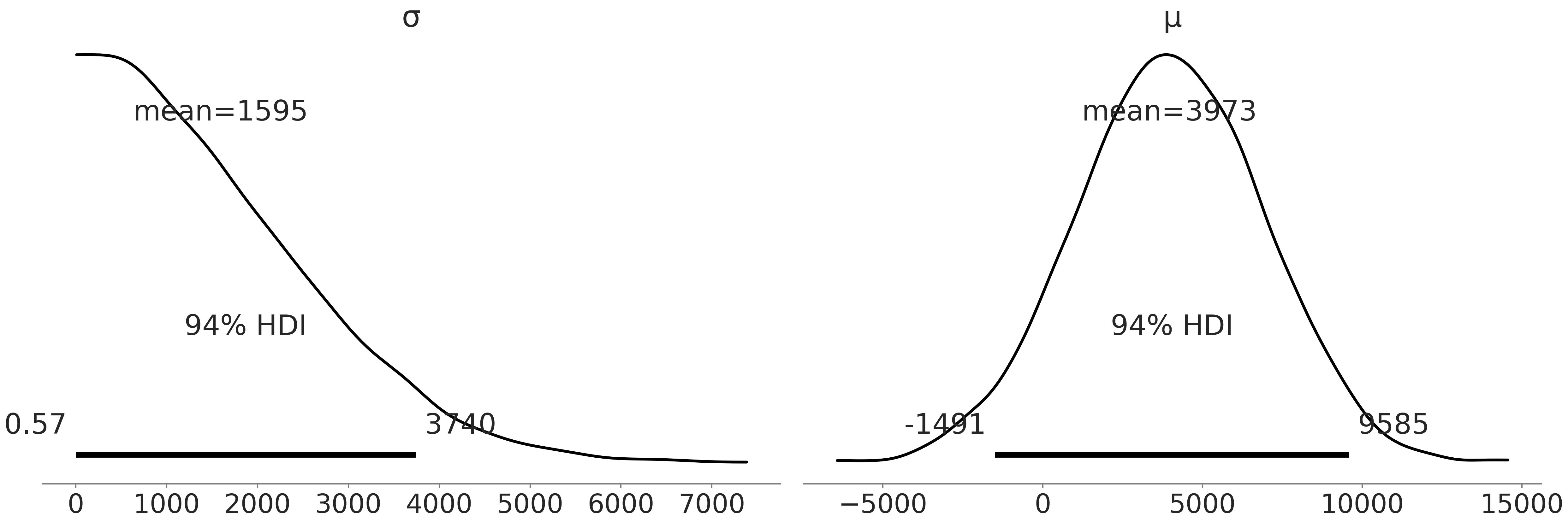
../_images/SingleSpecies_Prior_Predictive.png

Fig. 32 在代码 penguin_mass 中生成的先验样本。可以看出，企鹅体重的均值和标准差的分布估计涵盖了广泛的可能性。¶

从模型中做后验采样后，我们可以创建 Fig. 33，其中包括 $4$ 个子图，右边的两个是秩图，左边是参数的核密度估计，每条线为一个链。我们还可以参考 Table 4 中的数值诊断来了解采样链的收敛情况。根据第 2 章建立的直觉，我们大致能够判断该拟合可以接受，可以继续进行分析。

Table 4 企鹅体重的均值 (μ) 和标准差 (σ) 的贝叶斯估计，以及采样诊断。¶
	mean	sd	hdi_3%	hdi_97%	mcse_mean	mcse_sd	ess_bulk	ess_tail	r_hat
$\mu$	3707	38	3632	3772	0.6	0.4	3677.0	2754.0	1.0
$\sigma$	463	27	401	511	0.5	0.3	3553.0	2226.0	1.0

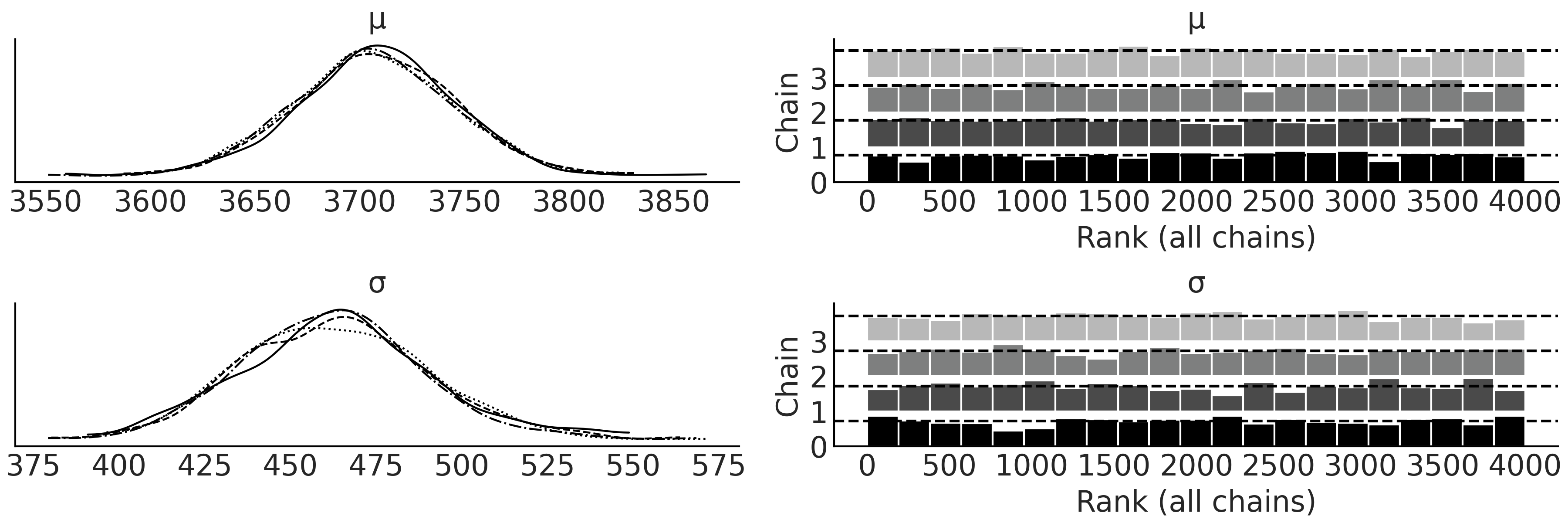
../_images/SingleSpecies_KDE_RankPlot.png

Fig. 33 代码 penguin_mass 中企鹅体重贝叶斯模型后验的核密度估计和秩图。该图用作采样的可视化诊断，以辅助判断在跨多个链的采样过程中是否存在问题。¶

为了理解拟合结果，我们在 Fig. 34 中绘制了一个结合所有链的后验图；并对 Table 3 中均值和标准差的点估计值做了标记，以便与贝叶斯估计值进行比较。

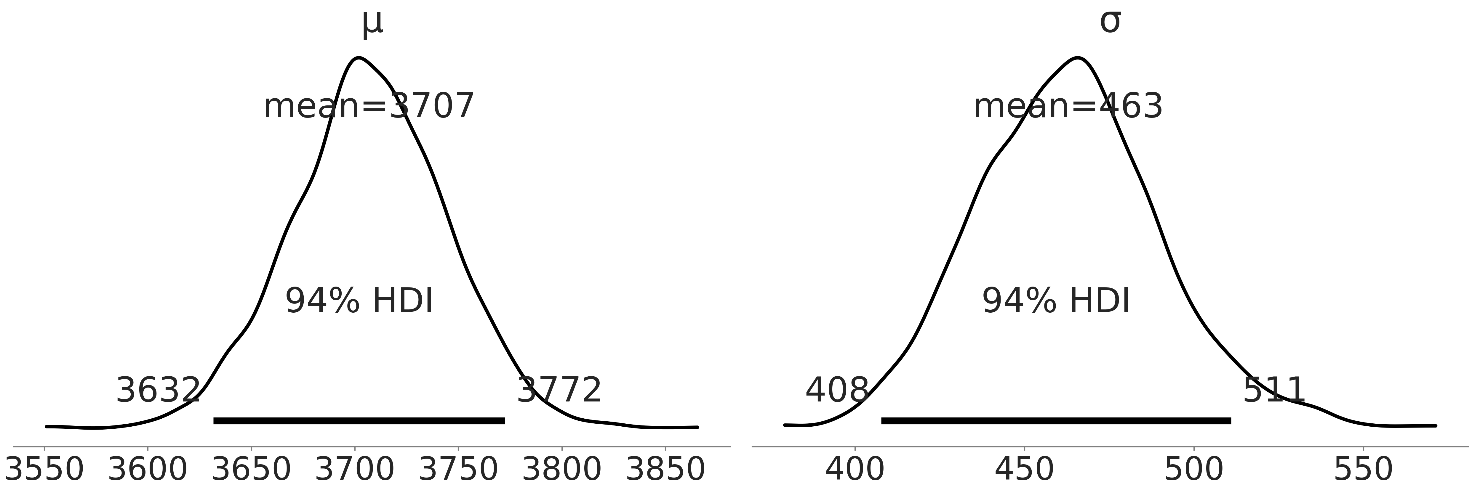
../_images/SingleSpecies_Mass_PosteriorPlot.png

Fig. 34 代码 penguin_mass 中，Adelie 种企鹅体重贝叶斯模型的后验分布图，其中，垂线是经验均值和标准差。¶

通过贝叶斯估计，我们得到了合理的参数分布。使用 Table 4 中的汇总信息，以及来自 Fig. 33 中的后验分布，该企鹅物种的体重均值从 $3632$ 到 $3772$ 克相当合理；此外边缘后验分布的标准差也比较大。

切记，后验分布是高斯分布参数（均值和标准差）的分布，而非高斯分布本身（即企鹅体重的分布），千万不要混淆。因此如果想要企鹅体重的分布估计，我们需要基于均值和标准差参数的后验样本生成后验预测分布。也就是说，根据当前模型设定，企鹅体重的分布应该是以 $\mu$ 和 $\sigma$ 的后验分布为条件的高斯分布。

现在已经描述了 Adelie 种企鹅的体重，我们可以继续对其他物种做同样的工作。在编程上，我们可以编写三个独立的模型来实现，但也可以只编写一个模型，其中包含 $3$ 个独立的组，每个物种对应一个组。

Listing 17 nocovariate_mass¶

# pd.categorical makes it easy to index species below
all_species = pd.Categorical(penguins["species"])

with pm.Model() as model_penguin_mass_all_species:
    # Note the addition of the shape parameter
    σ = pm.HalfStudentT("σ", 100, 2000, shape=3)
    μ = pm.Normal("μ", 4000, 3000, shape=3)
    mass = pm.Normal("mass",
                     mu=μ[all_species.codes],
                     sigma=σ[all_species.codes],
                     observed=penguins["body_mass_g"])

    trace = pm.sample()
    inf_data_model_penguin_mass_all_species = az.from_PyMC3(
        trace=trace,
        coords={"μ_dim_0": all_species.categories,
                "σ_dim_0": all_species.categories})

我们为每个参数使用了可选的 形状（ Shape ，Python 中描述多维张量各维度大小的术语） 参数，并在似然中添加一个索引，以告诉 PYMC3 我们希望独立调节每个物种的后验。在编程语言设计中，使表达思想更加无缝的小技巧被称为语法糖。概率编程开发人员也会使用一些语法糖；概率编程语言会努力让表达模型更容易且错误更少。

运行模型后，再次检查核密度估计曲线和秩图，参阅 Fig. 35。与 Fig. 33 相比，你将看到 $4$ 个额外的图，每个物种添加了 $2$ 个参数。花点时间将均值的估计与 Table 3 中各物种的汇总均值进行比较。为了更好地可视化各物种分布之间的差异，可以使用代码 mass_forest_plot 来绘制多个后验分布的森林图。

Fig. 36 使我们更容易对不同物种的估计做比较，注意 Gentoo 种企鹅 似乎比 Adelie 种 或 Chinstrap 种 有更大的体重。

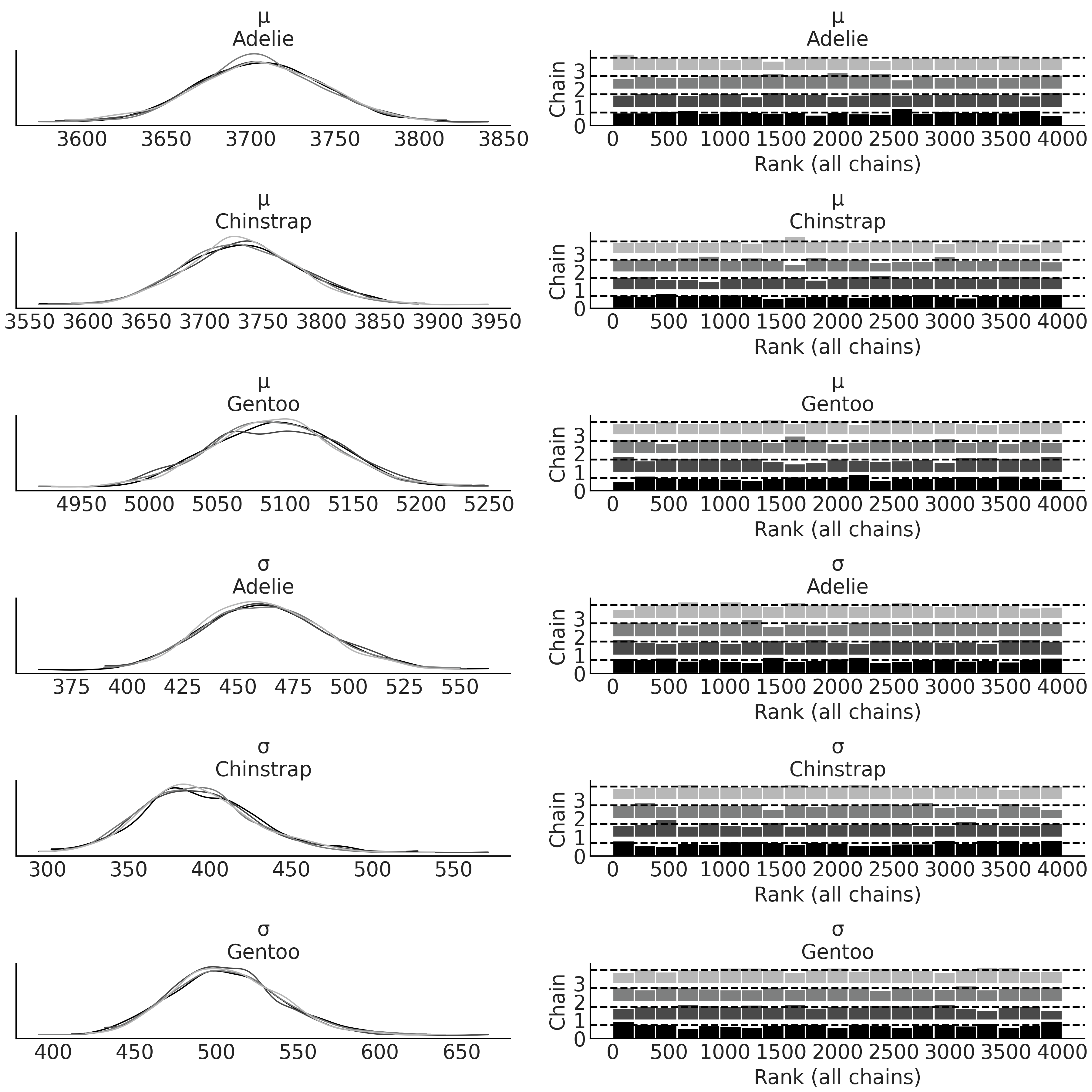
Fig. 35 penguins_masses 模型中的各种企鹅体重分布参数的后验估计核密度估计曲线和秩图。注意各物种都有自己的一对估计值。¶

Listing 18 mass_forest_plot¶

az.plot_forest(inf_data_model_penguin_mass_all_species, var_names=["μ"])

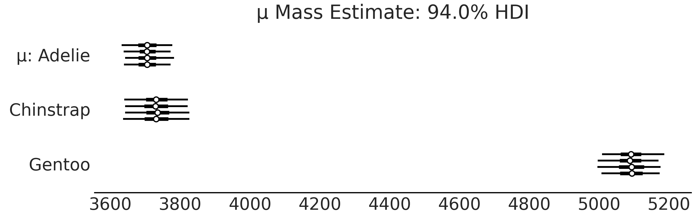
../_images/Independent_Model_ForestPlotMeans.png

Fig. 36 model_penguin_mass_all_species 中各物种组体重均值参数的后验森林图。每条线代表采样器中的一条链，点代表点估计，目前情况下指经验均值，细线是后验的 $25\%$ 到 $75\%$ 四分位数范围，粗线是 $94\%$ 最高密度区间 ( HDPI )。¶

Fig. 36 让我们更容易比较估计结果，并且很容易注意到 Gentoo 种企鹅的体重比 Adelie 种 或 Chinstrap 种 企鹅更大。让我们也看看 Fig. 37 中的标准差。后验的 $94\%$ 最高密度区间报告了大约存在 $100$ 克的不确定性。

az.plot_forest(inf_data_model_penguin_mass_all_species, var_names=["σ"]) 

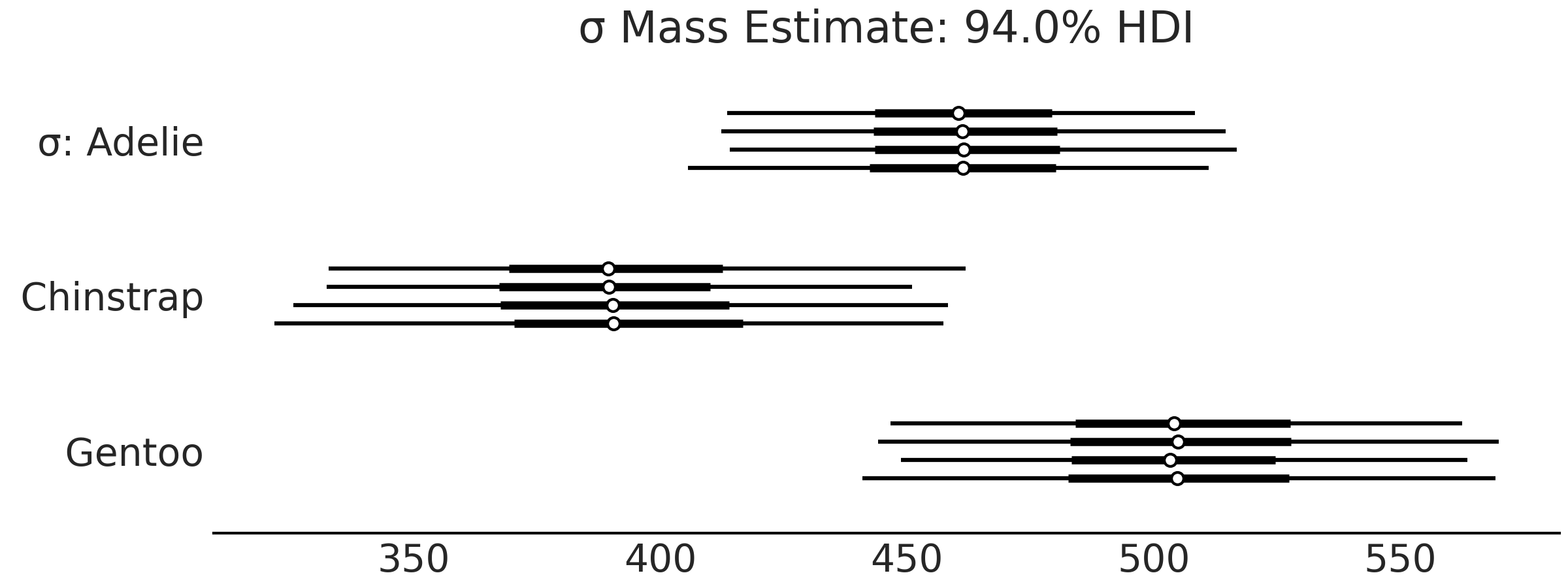
../_images/Independent_Model_ForestPlotSigma.png

Fig. 37 model_penguin_mass_all_species 中各物种组的体重标准差参数的后验森林图，描述了对各组企鹅体重离散度的估计，例如，给定 Gentoo 种企鹅体重分布均值的估计后，相关标准差可能在 $450$ 克到 $550$ 克之间。¶

3.1.1 比较两种概率编程语言¶

在进一步扩展统计建模思想之前，我们先花点时间讨论概率编程语言，并介绍将在本书中使用的另一种概率编程语言：TensorFlow Probability (TFP)。我们将在代码 nocovariate_mass 中，将 PYMC3 的截距模型转换为 TFP ，以便于大家理解。

学习不同的概率编程语言似乎没有必要。但本书中选择使用两种概率编程语言有些特殊的原因：在不同概率编程语言中看到相同的工作流程，将使你对贝叶斯建模和计算有更透彻的理解，帮助你将计算细节与统计思想分开，并使你成为一个更强大的建模者。

此外，不同概率编程语言有不同的能力和重点。 PYMC3 是更高级别的概率编程语言，可以轻松地以更少代码表达模型，而 TFP 为建模和推断提供了更低级别的概率编程能力。并非所有概率编程语言都能够像彼此一样非常容易地表达所有模型。例如，时间序列模型（第 6 章）在 TFP 中更容易定义，而贝叶斯加性回归树在 PYMC3 中更容易表达（第 7 章）。通过对多种语言的接触，你将对贝叶斯建模的基本要素以及其在在计算上的实现有更深入了解。

概率编程语言由原语组成，在编程语言中，原语是用于构建更复杂程序的最简单元素。你可以将原语理解成自然语言中的单词，能够形成更复杂的结构，比如句子。由于不同语言使用不同的词，不同概率编程语言也会使用不同的原语。这些原语主要用于表达模型、执行推断或表达工作流的其他部分。

在 PYMC3 中，与模型构建相关的原语包含在命名空间 pm 下。例如，在代码 penguin_mass 中，可以看到 pm.HalfStudentT(.) 和 pm.Normal(.)，其中“ $.$”代表一个随机变量。with pm.Model() as .语句调用 Python 的上下文环境管理器，PYMC3 使用该语句来收集上下文管理器中的随机变量，并构建模型model_adelie_penguin_mass。然后可以使用 pm.sample_prior_predictive(.)和pm.sample(.)` 分别获得先验预测分布和后验分布的样本。

类似地，TFP 为用户提供了在 tfp.distributions 中指定分布和模型、运行 MCMC 推断( tfp.mcmc ) 等原语。例如，为了构建贝叶斯模型，TensorFlow 提供了多个名为 tfd.JointDistribution 的 API 原语 [29]。在本书的其余部分中，我们会主要使用 tfd.JointDistributionCoroutine，但读者应当知道还有 tfd.JointDistribution 的一些变体可能更适合你的应用 1。由于导入数据和计算汇总统计量的代码和 penguin_load 和 penguin_mass_empirical 一致，因此这里我们专注于模型构建和推断。

model_penguin_mass_all_species 以 TFP 表示为代码 penguin_mass_tfp ：

Listing 19 penguin_mass_tfp¶

import tensorflow as tf
import tensorflow_probability as tfp

tfd = tfp.distributions
root = tfd.JointDistributionCoroutine.Root

species_idx = tf.constant(all_species.codes, tf.int32)
body_mass_g = tf.constant(penguins["body_mass_g"], tf.float32)

@tfd.JointDistributionCoroutine
def jd_penguin_mass_all_species():
    σ = yield root(tfd.Sample(
            tfd.HalfStudentT(df=100, loc=0, scale=2000),
            sample_shape=3,
            name="sigma"))
    μ = yield root(tfd.Sample(
            tfd.Normal(loc=4000, scale=3000),
            sample_shape=3,
            name="mu"))
    mass = yield tfd.Independent(
        tfd.Normal(loc=tf.gather(μ, species_idx, axis=-1),
                   scale=tf.gather(σ, species_idx, axis=-1)),
        reinterpreted_batch_ndims=1,
        name="mass")

这是我们第一次遇到用 TFP 编写的贝叶斯模型，所以花点时间来详细介绍一下。 tfp.distributions 是原语中的分布类，我们通常为其赋予一个较短的别名 tfd = tfp.distributions 。 tfd 中包含了常用的分布，例如高斯分布 tfd.Normal(.) 。代码中还使用了 tfd.Sample，它返回来自基础分布的多个独立副本（从概念上讲，实现了 PYMC3 语法糖 shape=(.) 的功能）。 tfd.Independent 用于指示该分布包含多少个副本，我们希望在计算对数似然时在某个轴上对这些副本求和，这由 reinterpreted_batch_ndims 函参指定。通常用 tfd.Independent 封装与观测相关的分布 2 。你可以在 10.8.1 PPL 中的形状处理部分阅读更多关于 TFP 和概率编程语言中的形状处理的信息。

代码中的模型签名 @tfd.JointDistributionCoroutine 很有意思，顾名思义，就是在 Python 中使用协程（ Coroutine ），不过我们在此不过多地介绍生成器和协程的概念。

yield 语句会为你提供模型函数内部的一些随机变量，你可以将 y = yield Normal(.) 视为 $y \sim \text{Normal(.)}$ 的代码表达方式。

此外，我们通过 tfd.JointDistributionCoroutine.Root 来包装没有依赖关系的随机变量。

该模型被编写为没有输入参数和返回值的 Python 函数，将 @tfd.JointDistributionCoroutine 放在 Python 函数之上作为装饰器，以方便直接获取模型（即 tfd.JointDistribution）。

结果的 jd_penguin_mass_all_species 是代码 nocovariate_mass 中的截距回归模型在 TFP 中的重写。它具有与其他 tfd.Distribution 类似的、可以在贝叶斯工作流中使用的方法。例如，抽取先验和先验预测样本可以调用 .sample(.) 方法，该方法返回一个类似于 namedtuple 的自定义嵌套 Python 结构体。在代码 penguin_mass_tfp_prior_predictive 中，我们抽取了 $10004 个先验和先验预测样本。

Listing 20 penguin_mass_tfp_prior_predictive¶

prior_predictive_samples = jd_penguin_mass_all_species.sample(1000)

tfd.JointDistribution 的 .sample(.) 方法也可以抽取条件样本，这也是将来抽取后验预测样本时采用的机制。你可以运行代码 penguin_mass_tfp_prior_predictive2 ，检查输出，查看将模型中某些随机变量被设置为特定值时，随机样本的变化情况。总体来说，我们在调用 .sample(.) 函数时，会调用前向的数据生成过程。

Listing 21 penguin_mass_tfp_prior_predictive2¶

jd_penguin_mass_all_species.sample(sigma=tf.constant([.1, .2, .3]))
jd_penguin_mass_all_species.sample(mu=tf.constant([.1, .2, .3]))

一旦将生成模型 jd_penguin_mass_all_species 调整为企鹅体重的观测值（即为模型指定数据），就能够获得模型参数的后验分布。

从计算角度来看，我们希望生成一个能够返回输入点处后验对数概率的函数。这可以通过创建 Python 函数闭包或使用 .experimental_pin 方法来实现，如代码 tfp_posterior_generation 所示：

Listing 22 tfp_posterior_generation¶

target_density_function = lambda *x: jd_penguin_mass_all_species.log_prob(
    *x, mass=body_mass_g)

jd_penguin_mass_observed = jd_penguin_mass_all_species.experimental_pin(
    mass=body_mass_g)
target_density_function = jd_penguin_mass_observed.unnormalized_log_prob

推断是使用 target_density_function 完成的，例如，我们可以找到函数的最大值，这给出了最大后验概率（MAP）估计。我们还可以使用 tfp.mcmc [30] 中的方法从后验采样。或者更方便的是，使用类似于 PYMC3 3 中当前使用的标准采样例程，如代码 tfp_posterior_inference 所示：

Listing 23 TFp 的后验推断¶

run_mcmc = tf.function(
    tfp.experimental.mcmc.windowed_adaptive_nuts,
    autograph=False, jit_compile=True)
mcmc_samples, sampler_stats = run_mcmc(
    1000, jd_penguin_mass_all_species, n_chains=4, num_adaptation_steps=1000,
    mass=body_mass_g)

inf_data_model_penguin_mass_all_species2 = az.from_dict(
    posterior={
        # TFP mcmc returns (num_samples, num_chains, ...), we swap
        # the first and second axis below for each RV so the shape
        # is what ArviZ expected.
        k:np.swapaxes(v, 1, 0)
        for k, v in mcmc_samples._asdict().items()},
    sample_stats={
        k:np.swapaxes(sampler_stats[k], 1, 0)
        for k in ["target_log_prob", "diverging", "accept_ratio", "n_steps"]}
)

在代码 tfp_posterior_inference 中，我们运行了 4 个 MCMC 链，每条链在 1000 个适应步骤后有 1000 个后验样本。在内部，它通过使用观测到的（附加关键字参数“mass=body_mass_g”最后）调节模型（作为参数传递给函数）来调用“experimental_pin”方法。

第 8-18 行将采样结果解析为 ArviZ InferenceData，我们现在可以在 ArviZ 中对贝叶斯模型进行诊断和探索性分析。我们还可以在下面的代码 tfp_idata_additional 中以透明的方式将先验和后验预测样本和数据对数似然添加到inf_data_model_penguin_mass_all_species2。请注意，我们使用了 tfd.JointDistribution 的 sample_distributions 方法，该方法抽取样本并生成以后验样本为条件的分布。

Listing 24 tfp_idata_additional¶

prior_predictive_samples = jd_penguin_mass_all_species.sample([1, 1000])
dist, samples = jd_penguin_mass_all_species.sample_distributions(
    value=mcmc_samples)
ppc_samples = samples[-1]
ppc_distribution = dist[-1].distribution
data_log_likelihood = ppc_distribution.log_prob(body_mass_g)

# Be careful not to run this code twice during REPL workflow.
inf_data_model_penguin_mass_all_species2.add_groups(
    prior=prior_predictive_samples[:-1]._asdict(),
    prior_predictive={"mass": prior_predictive_samples[-1]},
    posterior_predictive={"mass": np.swapaxes(ppc_samples, 1, 0)},
    log_likelihood={"mass": np.swapaxes(data_log_likelihood, 1, 0)},
    observed_data={"mass": body_mass_g}
)

我们对 TensorFlow Probability 的旋风之旅到此结束。像任何语言一样，你在初次接触时可能不会流利。但是通过比较这两个模型，你现在应该更好地了解哪些概念是以贝叶斯为中心，哪些概念是以概率编程语言为中心。在本章的剩余部分和下一章中，我们将在 PYMC3 和 TFP 之间切换，以继续帮助你识别这种差异并查看更多工作示例。我们包括将代码示例从一个翻译到另一个的练习，以帮助你在成为概率编程语言多语种的过程中进行练习。

3.2 线性回归¶

在上一节中，我们通过在高斯分布的均值和标准差参数上设置先验分布，来模拟企鹅体重的分布。特别是，我们假设了体重不会随数据中其他特征的变化而变化。不过，我们可能更希望通过已有的观测数据，能够预测企鹅的体重信息。直观地说，如果看到两只企鹅，其中一只长鳍、一只短鳍，那么即使手边没有设备来精确测量体重，我们也会认为长鳍企鹅会是那个体重较大的企鹅。利用鳍状肢长度来估计企鹅体重的最简单方法是拟合一个线性回归模型，其中体重的均值被 有条件 地建模为其他变量的线性组合：

(25)¶\[\begin{split}\begin{split} \mu =& \beta_0 + \beta_1 X_1 + \dots + \beta_m X_m \\ Y \sim& \mathcal{N}(\mu, \sigma) \end{split}\end{split}\]

其中系数由参数 $\beta_i$ 表示，其中 $\beta_0$ 是线性模型的截距； $X_i$ 被称为预测变量或协变量； $Y$ 被称为目标变量、输出、响应变量或因变量。公式中需要注意， $\boldsymbol{X}$ 和 $Y$ 都是观测数据，并且它们是成对的 $\{y_j, x_j\}$ （也就是说，如果改变 $Y$ 的顺序而不改变 $X$ 的顺序，将会破坏数据中的信息）。

上述模型我们称之为线性回归模型，因为其中参数（注意：并非预测变量）以线性方式被引入到模型中。对于具有单个预测变量的模型，我们可以将模型视为将一条线拟合到观测数据 $(X, y)$ ，对于更高维度，则可能是一个平面或超平面。

我们可以采用矩阵表示法表示公式 (25)：

(26)¶\[\mu = \mathbf{X}\boldsymbol{\beta} \]

这里用系数列向量 $\beta$ 和预测变量矩阵 $\mathbf{X}$ 之间的矩阵向量乘积表达了这种线性关系。在其他（非贝叶斯）场合中，你可能会看到另一种表达方式，将公式 (25) 重写为对线性预测的含噪声观测：

(27)¶\[Y = \mathbf{X}\boldsymbol{\beta} + \epsilon,\; \epsilon \sim \mathcal{N}(0, \sigma)\]

公式 (27) 将线性回归的确定性部分（线性预测）和随机部分（噪声）分开。不过公式 (25) 能够更清楚地展示出数据的生成过程。

Design Matrix

公式 (26) 中的矩阵 $\mathbf{X}$ 被称为设计矩阵，它是给定对象集的解释变量值的矩阵，加上一列表示截距的附加列。每行代表一个独特的观测结果（例如，企鹅），连续的列对应于变量（如 鳍状肢长度（ Flipper Length ） ）及其针对该对象的特定值。

设计矩阵不限于连续预测变量。对于类别型预测变量（即只有几个类别）的离散预测变量，将其转换为设计矩阵的常用方法称为虚拟编码（ Dummy Encoding ）或单热编码（ One Hot Encoding ）。例如，在企鹅截距模型（见代码 mass_forest_plot ）中，我们并没有使用 mu = μ[species.codes] ，而是使用 mu = pd.get_dummies(penguins["species"]) @ μ 将类别变量转换成了设计矩阵，其中 @ 是用于执行矩阵乘法的 Python 运算符。在 Python 中也有几个执行独热编码的函数，例如，sklearn.preprocessing.OneHotEncoder。

或者，可以对类别型预测变量进行编码，以使结果列和关联系数表示线性对比度。例如，两个类别型预测变量的不同设计矩阵编码与 ANOVA 的零假设检验设置中的 I、II 和 III 型平方和相关。

如果在 “三维空间” 中绘制公式 (25)，我们会得到 Fig. 38，它显示了结果变量按照似然函数的模型，随着观测数据 $x$ 的变化而变化。

需要说明的是，本章仅使用了线性关系来建模 $x$ 和 $Y$ 之间的关系，使用高斯分布作为似然。但在许多其他模型架构中，可能会有不同的选择，这一点在第 4 章中有所体现。

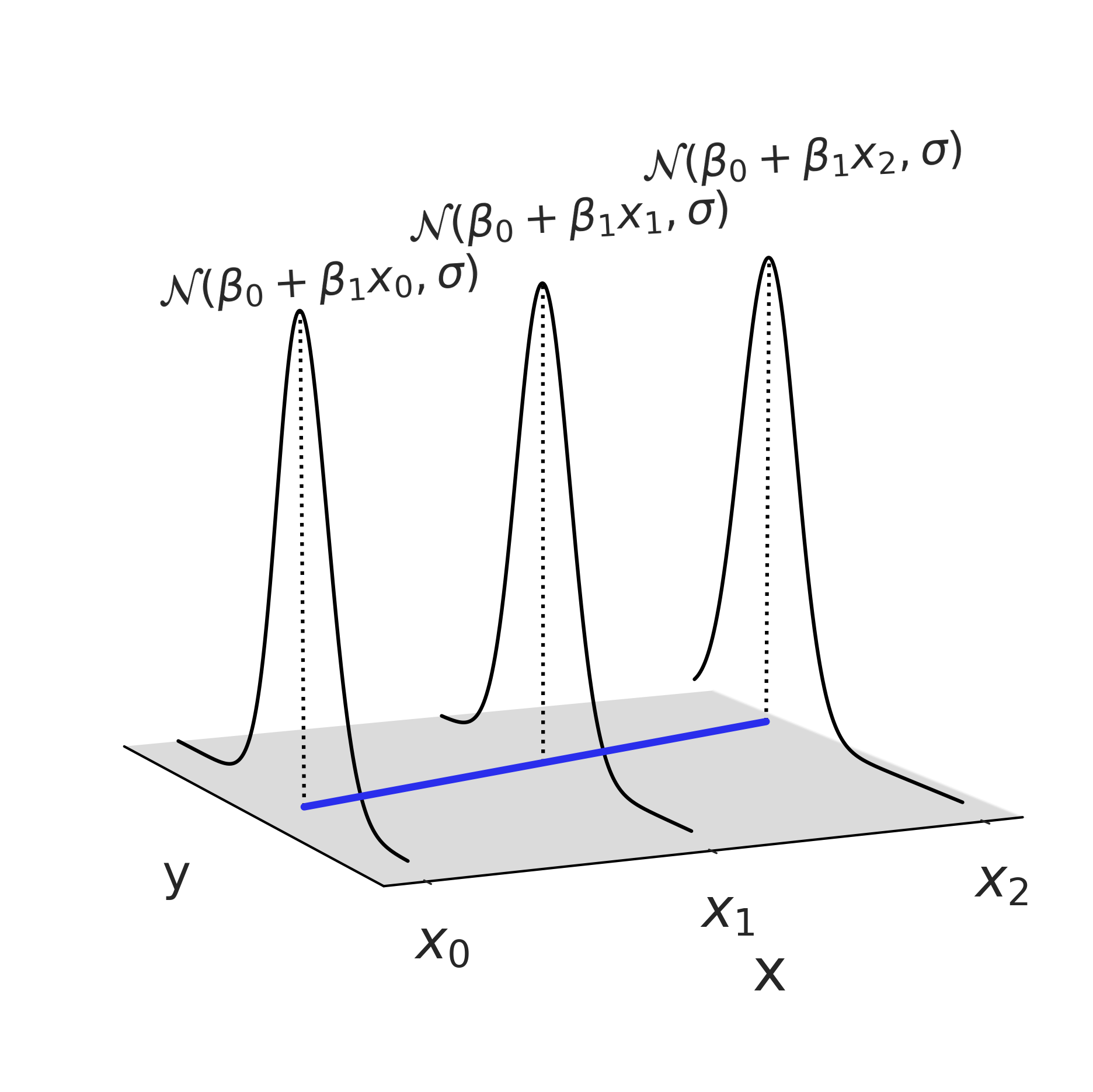
Fig. 38 在 $3$ 个点处评估了使用高斯似然的线性回归。此图仅显示了三个 $x$ 点处的一种可能的高斯分布（因为 $\beta_0,\beta_1,\sigma$ 都是随机变量）；在完成整个贝叶斯模型拟合后，将得到最终的高斯分布。不过该高斯分布的参数（即均值和标准差）并非一定要服从高斯分布。¶

3.2.1 一个简单的线性模型¶

如果回顾企鹅的例子，我们对使用鳍长度来估计和预测企鹅平均体重更感兴趣，可以在代码 non_centered_regression 中构建一个线性回归模型，其中包括两个新参数 $\beta_0$ 和 $\beta_1$ （通常称为截距和斜率）。对于此示例，代码中设置了 $\mathcal{N}(0, 4000)$ 的宽泛先验，这符合我们没有领域先验知识的假设。在运行采样器后，会估计出三个参数 $\sigma$ 、$\beta_1$ 和 $\beta_0$ 。

Listing 25 未做中心化处理的线性回归模型¶

adelie_flipper_length_obs = penguins.loc[adelie_mask, "flipper_length_mm"]

with pm.Model() as model_adelie_flipper_regression:
    # pm.Data allows us to change the underlying value in a later code block
    adelie_flipper_length = pm.Data("adelie_flipper_length",
                                    adelie_flipper_length_obs)
    σ = pm.HalfStudentT("σ", 100, 2000)
    β_0 = pm.Normal("β_0", 0, 4000)
    β_1 = pm.Normal("β_1", 0, 4000)
    μ = pm.Deterministic("μ", β_0 + β_1 * adelie_flipper_length)

    mass = pm.Normal("mass", mu=μ, sigma=σ, observed = adelie_mass_obs)

    inf_data_adelie_flipper_regression = pm.sample(return_inferencedata=True)

为了节省篇幅，本书中不会每次都展示诊断程序，但你不应盲目相信采样器。相反，你应该将运行诊断程序作为工作流程中的固定步骤，以验证你是否有可靠的近似后验。

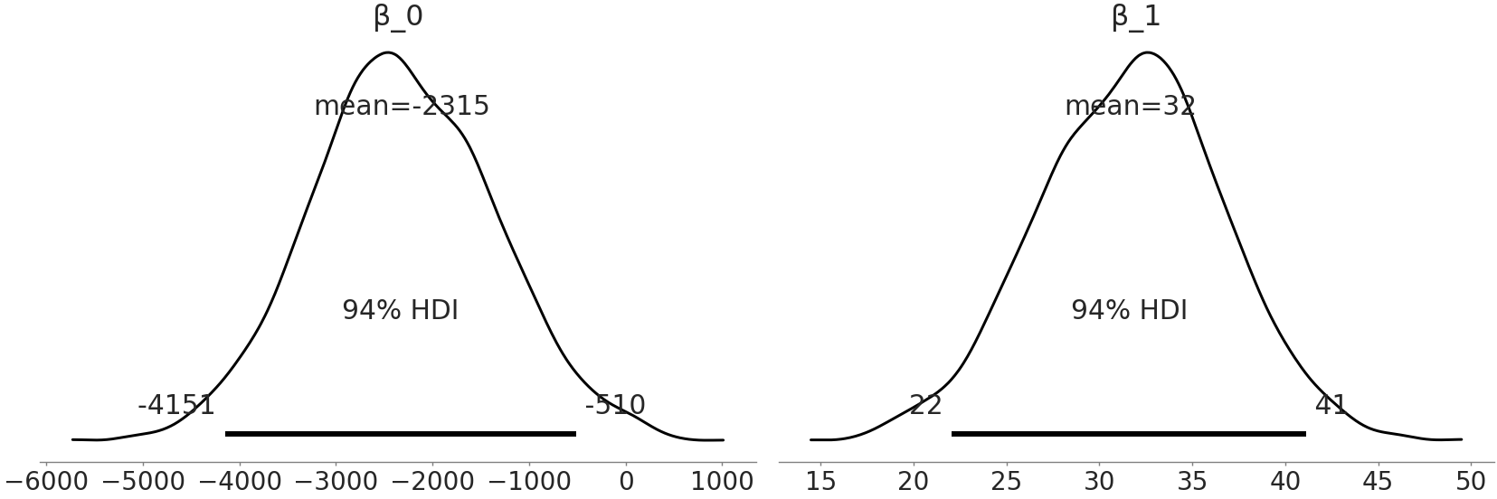
../_images/adelie_coefficient_posterior_plots.png

Fig. 39 model_adelie_flipper_regression 中系数的后验分布。¶

在采样器完成运行后，可以绘制参数的近似后验分布图 Fig. 39，其中显示了 $\beta_0$ 和 $\beta_1$ 的完整后验。

系数 $\beta_1$ 表示，对于 Adelie 种来说，鳍状肢长度的每毫米变化，理论上预计会平均产生 $32$ 克的体重变化，不过任何在 $22$ 克到 $41$ 克之间的变化值也都是可能发生的。此外，从 Fig. 39 中可以看到 $94\%$ 的最高密度区间未覆盖 $0$ 克，这表明体重和鳍状肢长度之间确实存在某种联系，支撑了我们的假设。此观察对于解释 “鳍状肢长度和体重之间的关系” 非常有用。但我们应该注意：不要过度解释系数，或认为线性模型必然意味着因果关系。例如，如果对一只企鹅进行鳍状肢的增肢手术，这会造成鳍长度增加，但不一定会造成体重增加。实际上，由于企鹅获取食物困难，体重反而可能降低。两者之间的逆向关系也不一定正确，给企鹅提供更多食物使其增重，这有助于其拥有更大的鳍状肢，但也可能使其成为一只更肥胖的企鹅。

现在看一下 $\beta_0$，它代表什么？根据后验估计结果，如果看到一只鳍状肢长度为 $0$ 毫米的Adelie 种企鹅，我们预计这只不存在的企鹅，体重在 $-4213$ 到 $-546$ 克之间。这个陈述按照模型来说是正确的，但负的体重并没有意义。这不一定是问题，没有规定模型中的每个参数都必须可解释，也没有规定模型对每个参数值都必须提供合理预测。

在当前情况下，上述特定模型的有限目的只是估计鳍状肢长度和企鹅体重之间的关系，通过后验估计，我们已经成功实现了这个目标。

模型: 数学和现实之间的平衡

在企鹅示例中，即使模型允许，企鹅体重低于 $0$（甚至接近 $0$ ）也是没有意义的。由于建模和拟合时使用了远离 $0$ 的体重值，所以当我们想要推断接近 $0$ 或低于 $0$ 的结果时，不应该对模型失败感到惊讶。模型不一定必须为所有可能的值提供合理预测，它只需要为构建它时的有限目的提供合理预测。

本节中，我们设想加入预测变量会更好地预测企鹅的体重。我们可以通过 Fig. 40 比较固定均值模型和线性变化均值模型的 $\sigma$ 后验估计来验证此设想，我们对似然的标准差估计已经从平均约 $460$ 克降到了 $380$ 克。

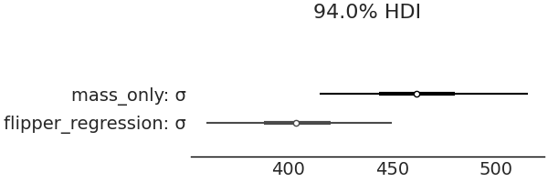
../_images/SingleSpecies_SingleRegression_Forest_Sigma_Comparison.png

Fig. 40 在估计企鹅体重时,通过使用鳍状肢长度作为预测变量，估计误差从略高于 $460$ 克的均值减少到大约 $380$ 克。直觉上这是有道理的，就像我们得到了关于估计量的信息，可以利用这些信息来做出更好的估计。¶

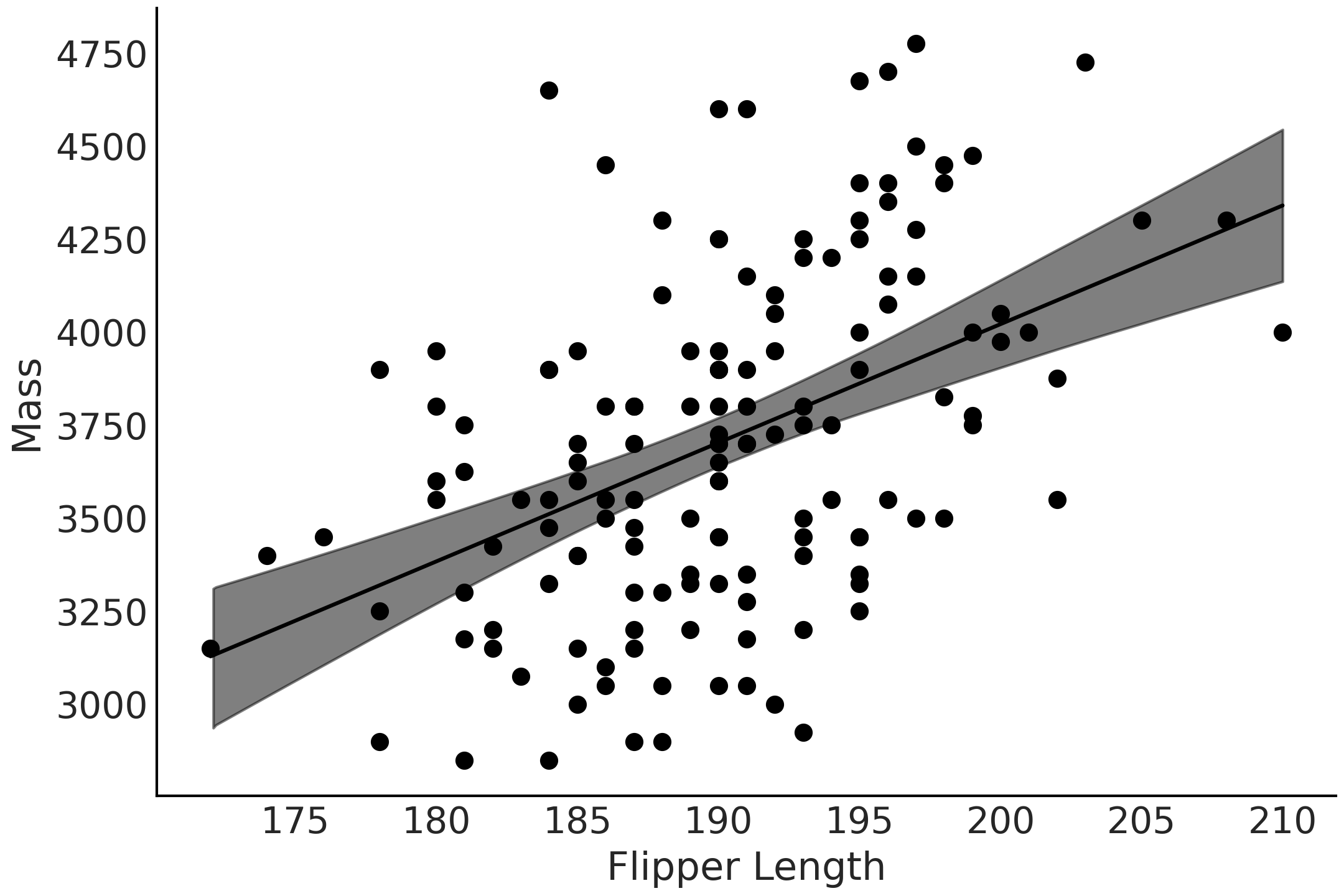
../_images/Flipper_length_mass_regression.png

Fig. 41 观测到的鳍状肢长度与 Adelie 种 的体重数据作散点图，似然的均值参数估计为黑线，均值参数的 $94\%$ HDI 为灰色区域。请注意均值在随鳍状肢长度变化而变化。¶

3.2.2 预测¶

在 3.2.1 一个简单的线性模型中，我们估计了鳍状肢长度和体重之间的线性关系。而回归的主要用途之一是利用此关系进行预测。在本例中，给定企鹅的鳍状肢长度，我们能够预测它的体重吗？当然可以！可以使用模型 model_adelie_flipper_regression 的推断结果来做预测。

在贝叶斯统计中，处理的对象都是概率分布，因此最终不会得到体重的单一预测值，而是所有可能体重值构成的分布。该分布就是公式 (6) 中定义的后验预测分布。

在实践中，我们通常不会（也可能无法）解析地计算预测分布，而是使用概率编程语言，利用后验分布的样本来估计预测值的分布（注：本质上是对模型参数的边缘化计算）。例如，如果有一只具有平均鳍状肢长度的企鹅，想预测其可能的体重，可以编写代码 penguins_ppd：

Listing 26 penguins_ppd¶

with model_adelie_flipper_regression:
    # Change the underlying value to the mean observed flipper length
    # for our posterior predictive samples
    pm.set_data({"adelie_flipper_length": [adelie_flipper_length_obs.mean()]})
    posterior_predictions = pm.sample_posterior_predictive(
        inf_data_adelie_flipper_regression.posterior, var_names=["mass", "μ"])

在代码 penguins_ppd 的第一行，我们将鳍状肢长度的值固定为观测数据中鳍状肢的平均长度。然后使用回归模型 model_adelie_flipper_regression，在该固定值处生成企鹅体重的后验预测样本。 Fig. 42 中绘制了具有平均鳍状肢长度的企鹅体重的后验预测分布。

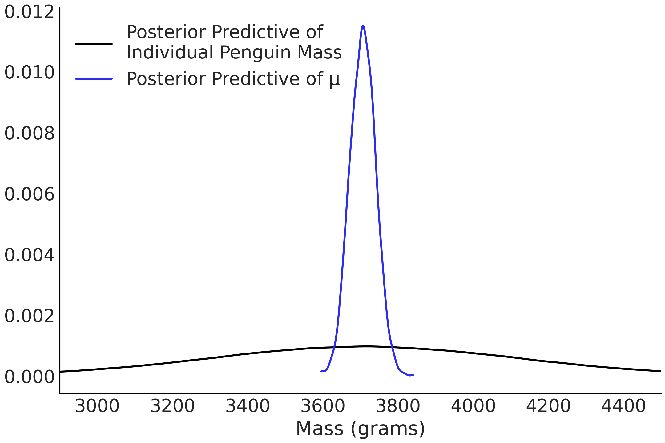
../_images/Flipper_length_mass_posterior_predictive.png

Fig. 42 在平均鳍状肢长度处评估的均值参数 $\mu$ 的后验分布，标记为蓝色；同时，在平均鳍状肢长度处评估的企鹅体重的后验预测分布标记为黑色。可以看出，黑色曲线更宽，因为它描述了（给定鳍状肢长度时）所以可能体重的分布（即均值参数和标准差参数的边缘化结果），而蓝色曲线仅表达了均值参数的分布（即均值的边缘分布）。¶

简而言之，我们不仅可以使用代码 non_centered_regression 中的模型来估计鳍状肢长度和企鹅体重之间的关系，还可以在任意鳍状肢长度处获得对应的企鹅体重估计分布。

换句话说，我们可以利用贝叶斯推断得出 $\beta_1$ 和 $\beta_0$ 系数，通过后验预测分布来预测任意鳍状肢长度对应的企鹅体重。

因此，后验预测分布在贝叶斯环境中是一个强大的工具，它不仅让我们可以预测最可能的值，还可以预测包含不确定性的合理值的分布，如公式 (6) 。

3.2.3 中心化处理¶

代码 non_centered_regression 中的模型在估计鳍状肢长度和企鹅体重之间的关系，以及预测给定鳍状肢长度下的企鹅体重方面效果很好。遗憾的是，数据和模型对 $\beta_0$ 的估计并不是特别有意义，因此我们可以通过数据转换来使 $\beta_0$ 更易于解释。通常我们会选择中心化处理，即采纳一组数据并将其均值中心化为零，如代码 flipper_centering 所示。

Listing 27 flipper_centering¶

adelie_flipper_length_c = (adelie_flipper_length_obs -
                           adelie_flipper_length_obs.mean())

使用中心化后的预测变量再次拟合模型，这次使用 TFP。

Listing 28 tfp_penguins_centered_predictor¶

def gen_adelie_flipper_model(adelie_flipper_length):
    adelie_flipper_length = tf.constant(adelie_flipper_length, tf.float32)

    @tfd.JointDistributionCoroutine
    def jd_adelie_flipper_regression():
        σ = yield root(
            tfd.HalfStudentT(df=100, loc=0, scale=2000, name="sigma"))
        β_1 = yield root(tfd.Normal(loc=0, scale=4000, name="beta_1"))
        β_0 = yield root(tfd.Normal(loc=0, scale=4000, name="beta_0"))
        μ = β_0[..., None] + β_1[..., None] * adelie_flipper_length
        mass = yield tfd.Independent(
            tfd.Normal(loc=μ, scale=σ[..., None]),
            reinterpreted_batch_ndims=1,
            name="mass")

    return jd_adelie_flipper_regression

# If use non-centered predictor, this will give the same model as
# model_adelie_flipper_regression
jd_adelie_flipper_regression = gen_adelie_flipper_model(
    adelie_flipper_length_c)

mcmc_samples, sampler_stats = run_mcmc(
    1000, jd_adelie_flipper_regression, n_chains=4, num_adaptation_steps=1000,
    mass=tf.constant(adelie_mass_obs, tf.float32))

inf_data_adelie_flipper_length_c = az.from_dict(
    posterior={
        k:np.swapaxes(v, 1, 0)
        for k, v in mcmc_samples._asdict().items()},
    sample_stats={
        k:np.swapaxes(sampler_stats[k], 1, 0)
        for k in ["target_log_prob", "diverging", "accept_ratio", "n_steps"]}
)

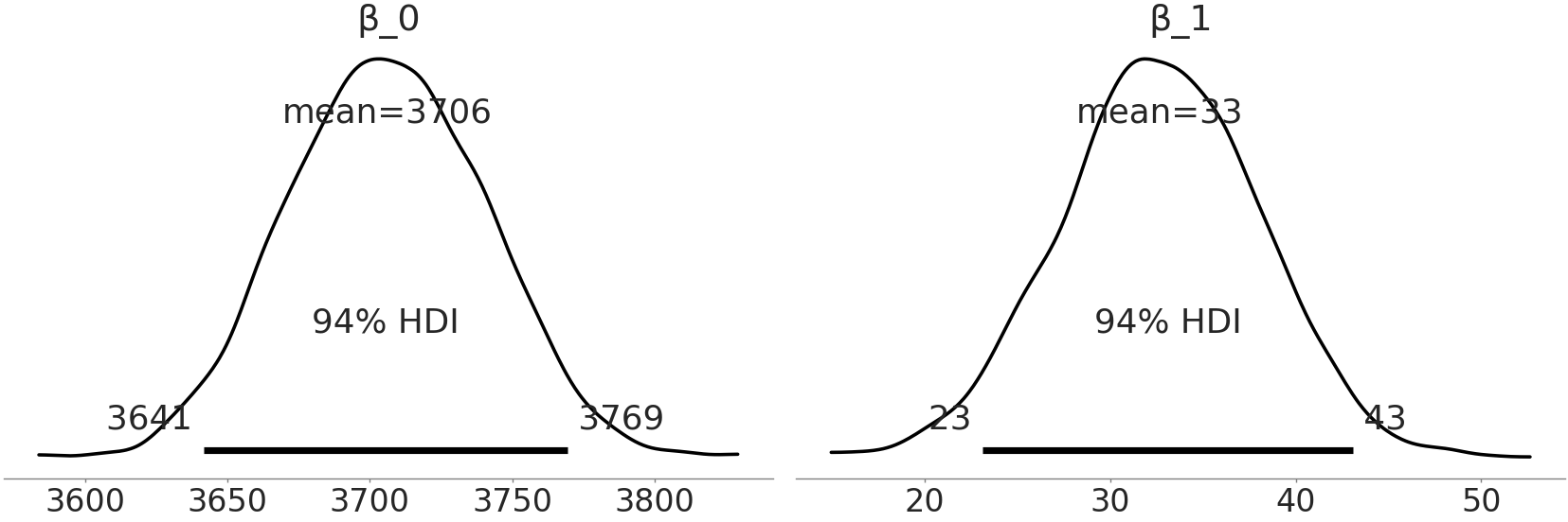
../_images/SingleSpecies_MultipleRegression_Centered.png

Fig. 43 来自代码 tfp_penguins_centered_predictor 的系数估计。注意，$beta\_1$ 的分布与 Fig. 39 中相同，但 $beta\_0$ 的分布发生了偏移。由于我们在鳍状肢长度的均值处做了中心化处理，因此 $beta\_0$ 现在代表了具有平均鳍状肢长度的企鹅体重分布。¶

代码 tfp_penguins_centered_predictor 中定义的数学模型与代码 non_centered_regression 中的 PYMC3 模型 model_adelie_flipper_regression 基本等价，唯一区别是对预测变量做了中心化处理。不过，在概率编程语言方面，TFP 的结构需要在不同行中添加 tensor_x[..., None] 来扩展标量的批次，使其能够与向量批次一起广播。具体来说，None 会添加一个新轴，这也可以使用 np.newaxis 或 tf.newaxis 来完成。此外，TFP 还将模型包装在一个函数中，以便轻松地将不同的预测变量作为条件。当然，中心化处理后，预测变量也应当是中心化后的变量。

当再次绘制系数的后验分布时，$\beta_1$ 与 PYMC3 模型相同，但 $\beta_0$ 的分布发生了变化。由于我们将输入数据中心化到了其均值上，$\beta_0$ 的后验分布将代表非中心化数据集中均值对应的预测分布。通过将数据中心化，现在可以将 $\beta_0$ 解释为具有平均鳍状肢长度的 Adelie 种企鹅的平均体重分布。

转换输入变量的想法也可以在任意选择的值上执行。例如，可以减去最小鳍状肢长度后拟合模型。在做这种转换后，可以将 $\beta_0$ 的解释变更为观测到的最小鳍状肢长度的平均体重分布。

为了更深入地讨论线性回归中的转换，推荐应用回归分析和广义线性模型 [31]。

3.3 多元线性回归¶

在许多物种中，不同性别之间存在双态性或差异。企鹅性别的双态性研究是收集 Palmer Penguin 数据集 [32] 的出发点之一。为了更仔细地研究企鹅的双态性，数据集中添加了第二个预测变量：性别（ sex ），并将其编码为二值型类别变量，现在来看我们是否可以更精确地估计企鹅的体重。

Listing 29 penguin_mass_multi¶

# Binary encoding of the categorical predictor
sex_obs = penguins.loc[adelie_mask ,"sex"].replace({"male":0, "female":1})

with pm.Model() as model_penguin_mass_categorical:
    σ = pm.HalfStudentT("σ", 100, 2000)
    β_0 = pm.Normal("β_0", 0, 3000)
    β_1 = pm.Normal("β_1", 0, 3000)
    β_2 = pm.Normal("β_2", 0, 3000)

    μ = pm.Deterministic(
        "μ", β_0 + β_1 * adelie_flipper_length_obs + β_2 * sex_obs)

    mass = pm.Normal("mass", mu=μ, sigma=σ, observed=adelie_mass_obs)

    inf_data_penguin_mass_categorical = pm.sample(
        target_accept=.9, return_inferencedata=True)

你会注意到新参数 $\beta_{2}$ 对体重的期望 $\mu$ 也有贡献。由于性别是一个类别型预测变量（本例中为 male 和 female ），我们将其分别编码为 $0$ 和 $1$。代码中的模型意味着：对于雌性企鹅来说，$\mu$ 的值是 $3$ 个项的总和；而对于雄性企鹅来说，是两个项的总和（因为 $\beta_2$ 项将被性别的取值归零）。

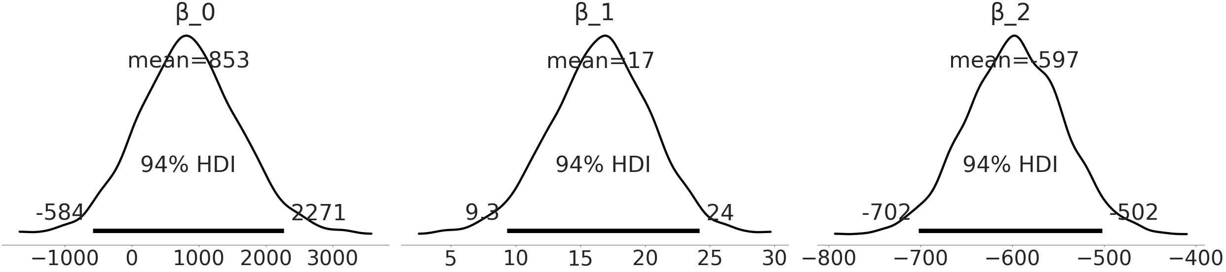
../_images/adelie_sex_coefficient_posterior.png

Fig. 44 估计模型中的性别预测变量系数 $\beta_{2}$ 。雄性企鹅编码为 $0$，雌性企鹅编码为 $1$ ，这表示我们认可：具有相同鳍状肢长度的雄性和雌性 Adelie 种 企鹅之间存在额外的体重差别。¶

线性模型的语法糖

线性模型的使用如此广泛，以至于有人为其回归专门编写了语法、方法和库。其中一个典型库是 Bambi（贝叶斯模型构建接口，Bayesian Model-Building Interface 的缩写）[33]）。

Bambi 是一个 Python 软件包，使用形式化语法来拟合广义线性层次模型，类似于在 R 包中的 lme4 包 [34]、nlme 包 [35]、rstanarm 包 [36] 或 brms 包 [37]）等。

Bambi 在底层使用 PYMC3 并提供更高级别的 API。要编写同一个模型，在忽略代码 penguin_mass_multi 中的先验 4 时，可以用 Bambi 编程为：

Listing 30 bambi_categorical¶

import bambi as bmb
model = bmb.Model("body_mass_g ~ flipper_length_mm + sex",
                  penguins[adelie_mask])
trace = model.fit()

如果不人为设置先验，软件包会自动分配先验。在 Bambi 内部几乎存储了 PYMC3 生成的所有对象，使用户可以轻松检索、检查和修改这些对象。此外，Bambi 还返回一个 az.InferenceData 对象，可以直接与 ArviZ 一起使用。

由于我们将 “雄性” 编码为 $0$，因此来自 model_penguin_mass_categorical 的后验估计了雄性企鹅与具有相同鳍状肢长度的雌性企鹅相比的体重差异。这里比较重要的一点是：模型通过引入第二个预测变量，形成了一个多元线性回归，同时我们在解释系数时也必须更加小心了。在多元线性回归中，系数通常提供了如下信息：如果所有其他预测变量保持不变时，某个预测变量与结果变量之间的线性关系 5。

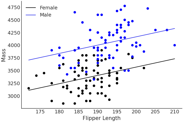
../_images/Single_Species_Categorical_Regression.png

Fig. 45 使用类别型预测变量编码的雄性和雌性 Adelie 种 企鹅的鳍状肢长度与体重之间的多元回归。注意雄性和雌性企鹅之间的体重差异所有鳍状肢长度上保持不变，该差异相当于 $\beta_2$ 系数的大小。¶

我们可以再次在 Fig. 46 中比较三个模型的标准差，看看是否减少了估计中的不确定性。可以看出，额外提供的信息进一步改进了估计。在当前情况下，我们对 $\sigma$ 的估计从无预测变量模型中的平均 $462$ 克下降到了多元线性模型中的平均 $298$ 克。这种不确定性的减少表明，性别确实为估计企鹅体重提供了有用信息。

Listing 31 forest_multiple_models¶

az.plot_forest([inf_data_adelie_penguin_mass,
        inf_data_adelie_flipper_regression,
        inf_data_penguin_mass_categorical],
        var_names=["σ"], combined=True)

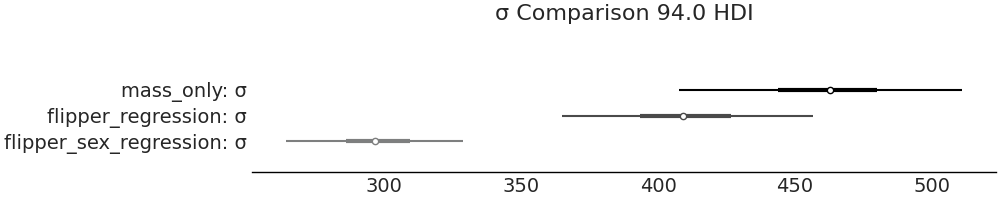
../_images/SingleSpecies_MultipleRegression_Forest_Sigma_Comparison.png

Fig. 46 将性别作为预测变量纳入 model_penguin_mass_categorical 中，可以观察到，该模型中 $\sigma$ 参数的估计值以 $300$ 克为中心，远低于无预测变量模型和单预测变量模型的估计结果，说明新模型的不确定性有减少。该图由代码 forest_multiple_models 生成。¶

更多的预测变量（或协变量）并非总是好事

模型拟合算法能够拟合所有观测信号（即便该信号是一个随机噪声信号）的现象，被称为产生了过度拟合（简称过拟合）。过拟合描述了一种情况，即算法可以很容易地将预测变量映射到已知案例中的结果，但无法推广到新的数据。在线性回归中，我们可以随机地生成 $100$ 个预测变量，并将它们拟合到随机的模拟数据集上，能够很好地证明这种现象 [10] 。结果会表明，即便预测变量和结果变量之间完全随机且没有任何关系，最终也会归纳出一个对已有数据做得非常好的模型。

3.3.1 反事实分析¶

在一元回归的代码 penguins_ppd 中，我们使用拟合的参数进行预测，调整鳍状肢长度以获得相应的体重估计。在多元回归中，可以做类似的工作。我们可以保持其他所有预测变量固定，然后查看剩下的那个预测变量和结果变量之间的关系。此分析方法通常被称为反事实分析（ Counterfactual Analysis）。

让我们扩展上一节代码 penguin_mass_multi 的多元回归，这次增加喙长度（ Bill Length ），并在 TFP 中运行反事实分析。模型构建和推断见代码 tfp_flipper_bill_sex 。

Listing 32 tfp_flipper_bill_sex¶

def gen_jd_flipper_bill_sex(flipper_length, sex, bill_length, dtype=tf.float32):
    flipper_length, sex, bill_length = tf.nest.map_structure(
        lambda x: tf.constant(x, dtype),
        (flipper_length, sex, bill_length)
    )

    @tfd.JointDistributionCoroutine
    def jd_flipper_bill_sex():
        σ = yield root(
            tfd.HalfStudentT(df=100, loc=0, scale=2000, name="sigma"))
        β_0 = yield root(tfd.Normal(loc=0, scale=3000, name="beta_0"))
        β_1 = yield root(tfd.Normal(loc=0, scale=3000, name="beta_1"))
        β_2 = yield root(tfd.Normal(loc=0, scale=3000, name="beta_2"))
        β_3 = yield root(tfd.Normal(loc=0, scale=3000, name="beta_3"))
        μ = (β_0[..., None]
             + β_1[..., None] * flipper_length
             + β_2[..., None] * sex
             + β_3[..., None] * bill_length
            )
        mass = yield tfd.Independent(
            tfd.Normal(loc=μ, scale=σ[..., None]),
            reinterpreted_batch_ndims=1,
            name="mass")

    return jd_flipper_bill_sex

bill_length_obs = penguins.loc[adelie_mask, "bill_length_mm"]
jd_flipper_bill_sex = gen_jd_flipper_bill_sex(
    adelie_flipper_length_obs, sex_obs, bill_length_obs)

mcmc_samples, sampler_stats = run_mcmc(
    1000, jd_flipper_bill_sex, n_chains=4, num_adaptation_steps=1000,
    mass=tf.constant(adelie_mass_obs, tf.float32))

在该模型中，添加了另一个系数 beta_3 对应于预测变量喙长度。推断完成后，我们可以固定企鹅性别为雄性、喙长度为数据集均值，然后模拟具有不同鳍状肢长度的企鹅体重。这在代码 tfp_flipper_bill_sex_counterfactuals 中实现，结果见 Fig. 47 。由于将模型生成过程封装在了 Python 函数中（一种函数式编程风格的方法），因此很容易在新预测变量上做条件化，这对于反事实分析非常有用。

Listing 33 tfp_flipper_bill_sex_counterfactuals¶

mean_flipper_length = penguins.loc[adelie_mask, "flipper_length_mm"].mean()
# Counterfactual dimensions is set to 21 to allow us to get the mean exactly
counterfactual_flipper_lengths = np.linspace(
    mean_flipper_length-20, mean_flipper_length+20, 21)
sex_male_indicator = np.zeros_like(counterfactual_flipper_lengths)
mean_bill_length = np.ones_like(
    counterfactual_flipper_lengths) * bill_length_obs.mean()

jd_flipper_bill_sex_counterfactual = gen_jd_flipper_bill_sex(
    counterfactual_flipper_lengths, sex_male_indicator, mean_bill_length)
ppc_samples = jd_flipper_bill_sex_counterfactual.sample(value=mcmc_samples)
estimated_mass = ppc_samples[-1].numpy().reshape(-1, 21)

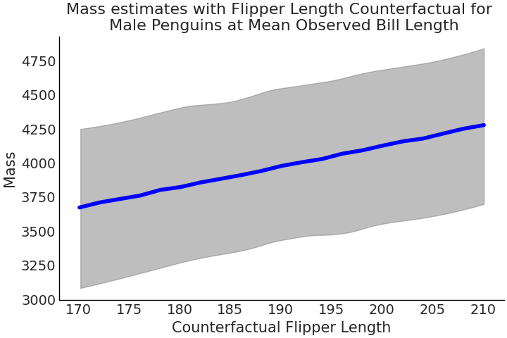
Fig. 47 代码 tfp_flipper_bill_sex_counterfactuals 中，采用反事实分析方法获得的 Adelie 种 企鹅的体重估计值，其中仅鳍状肢长度变化，所有其他预测变量都保持不变。¶

遵循 McElreath[10] 的提法， Fig. 47 被称为反事实图。正如 “反事实” 一词所暗示的那样，我们正在评估一种与观测数据或事实相悖的情况。或者换句话说，我们正在评估尚未发生的情况。

反事实图的用途之一是通过调整预测变量来探索结果变量的预测值。这是一种很棒的方法，因为它使我们能够探索现实中无法实现的一些 what-if 场景 6。但是，在解释这种方法时我们必须谨慎，因为可能存在一些陷阱。第一个陷阱是反事实的结果有可能根本不会出现，例如，永远不会存在鳍状肢长度大于 $1500$ 毫米的企鹅，但该模型会机械地提供对这种情况的估计。第二个陷阱更隐蔽，即假设可以独立地改变每个预测变量。这在实际中几乎不可能出现。例如，随着企鹅鳍状肢长度的增加，其他预测变量（如喙长度）也会增加。

反事实分析法的强大之处在于：其允许我们探索尚未发生的结果，或者至少没有被观测到发生的结果；但该方法也很容易为永远不会发生的情况生成估计值。模型本身无法区分两者，只能由建模者来识别它们。

相关性（ Correlation ）与因果性（ Causality ）

在解释线性回归时，很容易将其描述为 “ $X$ 的增加导致了 $Y$ 的增加 ” （即 $Y$ 是 $X$ 的结果），但事实并不一定如此。事实上 因果陈述 无法仅从回归关系中得出。在数学上，回归模型只是将两个（或更多变量）联系在一起，但这种联系不需要是因果关系。例如，增加降水量可以（并且因果地）促进植物的生长，但没有什么能够阻止我们颠倒这种关系，即用植物的生长来估计降水量，尽管我们都知道植物的生长不会导致降雨 7。

因果推断涉及在随机实验或观测研究背景下做出因果陈述所必需的一些工具和程序，感兴趣的读者可以参见第 7 章中的简要讨论。

3.4 广义线性模型¶

到目前为止，我们讨论的所有线性模型都假设观测值的分布为高斯分布，这在许多情况下都能很好地工作。但有时我们可能需要使用其他分布。例如要对受限于某个区间的事物建模，区间 $[0, 1]$ 中的数字类似于概率，或者自然数 $\{1, 2, 3, \dots \}$ 类似于计数事件。为此，我们使用线性函数 $\mathbf{X} \mathit{\beta}$，并使用反向链接函数 8 $\phi$ 对其进行修改，如公式 (28) 所示：

(28)¶\[\begin{split}\begin{split} \mu =& \phi(\mathbf{X} \beta) \\ Y \sim& \Psi (\mu, \theta) \end{split}\end{split}\]

其中 $\Psi$ 是一些由 $\mu$ 和 $\theta$ 参数化的分布，表示数据的似然。

反向链接函数的具体目的是将实数范围 $(-\infty, \infty)$ 的输出映射到受限区间范围。换句话说，反向链接函数是将线性模型推广到更多模型架构所需的一种 “技巧”。我们在这里处理的仍然是线性模型，因为生成观测数据的分布（即似然）均值仍然遵循模型参数和预测变量之间的线性函数，只不过现在可以将其使用和推广到更多场景 9。

3.4.1 结果变量取值为概率时 — 逻辑斯谛回归¶

最常见的广义线性模型之一是逻辑斯谛回归。它在只有两种可能结果之一的数据建模中特别有用。掷硬币中“正面”或“反面”结果的概率是常见的教科书示例。更多“现实世界”中的例子包括：生产中的缺陷可能性、癌症测试的阴性或阳性、火箭发射是否失败 [38]。

在逻辑斯谛回归中，反向链接函数被称为 逻辑斯谛函数（ logistic function ），它将 $(-\infty, \infty)$ 映射到 $(0,1)$ 区间。这很方便，因为现在我们可以将线性函数映射到概率值的 $0$ 到 $1$ 范围内。

(29)¶\[p = \frac{1}{1+e^{-\mathbf{X}\beta}}\]

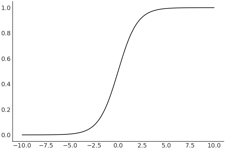
Fig. 48 一个逻辑斯谛函数示例图。请注意，结果变量已被“压缩”到区间 (0,1) 中。¶

通过逻辑斯谛回归，我们能够使用线性模型来估计事件的概率。有时，我们想要对给定数据进行分类或预测，此时我们希望将区间 $(-\infty, \infty)$ 内的某个连续预测值转换至 $0$ 到 $1$ 之间。然后，可以使用决策边界将其划分为集合 $\{0 ,1\}$ 中的某一个元素。假设将决策边界设置为 $0.5$ 的概率，则对于具有截距和单预测变量的模型，我们有：

\[\begin{split}\begin{split} 0.5 &= logistic(\beta_{0} + \beta_{1}*x) \\ logit(0.5) &= \beta_{0} + \beta_{1}*x \\ 0 &= \beta_{0} + \beta_{1}*x \\ x &= -\frac{\beta_{0}}{\beta_{1}} \\ \end{split}\end{split}\]

请注意，$logit$ 是 $logistic$ 的逆函数。也就是说，一旦拟合了逻辑斯谛模型，我们就可以使用系数 $\beta_0$ 和 $\beta_1$ 轻松计算出类概率大于 $0.5$ 的 $x$ 值。

3.4.2 结果变量为类别变量时 — 分类模型¶

在前面部分中，我们使用企鹅性别和喙长度来估计企鹅的体重。现在改变以下该问题：如果给定企鹅的体重、性别和喙长，我们能够预测其物种吗？

让我们使用 Adelie和 Chinstrap 这两个企鹅物种来完成此二元任务。就像上次一样，首先使用一个简单模型，只有一个预测变量，即喙长度。我们在代码 model_logistic_penguins_bill_length 中编写这个逻辑斯谛模型：

Listing 34 model_logistic_penguins_bill_length¶

species_filter = penguins["species"].isin(["Adelie", "Chinstrap"])
bill_length_obs = penguins.loc[species_filter, "bill_length_mm"].values
species = pd.Categorical(penguins.loc[species_filter, "species"])

with pm.Model() as model_logistic_penguins_bill_length:
    β_0 = pm.Normal("β_0", mu=0, sigma=10)
    β_1 = pm.Normal("β_1", mu=0, sigma=10)

    μ = β_0 + pm.math.dot(bill_length_obs, β_1)

    # A`PPL`ication of our sigmoid  link function
    θ = pm.Deterministic("θ", pm.math.sigmoid(μ))

    # Useful for plotting the decision boundary later
    bd = pm.Deterministic("bd", -β_0/β_1)

    # Note the change in likelihood
    yl = pm.Bernoulli("yl", p=θ, observed=species.codes)

    prior_predictive_logistic_penguins_bill_length = pm.sample_prior_predictive()
    trace_logistic_penguins_bill_length = pm.sample(5000, chains=2)
    inf_data_logistic_penguins_bill_length = az.from_PyMC3(
        prior=prior_predictive_logistic_penguins_bill_length,
        trace=trace_logistic_penguins_bill_length)

在广义线性模型中，从参数先验到响应值的映射有时难以理解，此时可以利用先验预测样本来帮助我们可视化预期的观测结果，这被称之为先验预测检查。

在企鹅分类的例子中，通过先验预测检查可以发现：在看到任何数据之前，在所有喙长度上属于 Gentoo 种 和 Adelie 种 的预期都是合理的。我们通过先验预测检查可以双重检查先验设置和模型是否能够切实表达我们的建模意图。在看到数据之前， Fig. 49 中这些类大致上是均匀的，这也是我们所期望的。

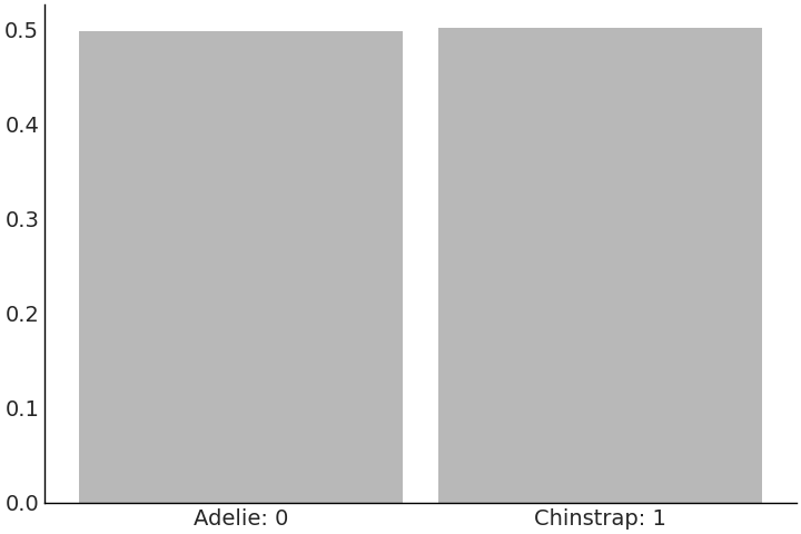
../_images/Prior_Predictive_Logistic.png

Fig. 49 来自 model_logistic_penguins_bill_length 的 $5000$ 个关于类别预测的先验预测样本。这种似然是离散的，更具体地说是二值的，与之前模型中估计的连续型的企鹅体重有所不同。¶

在模型中拟合出参数后，我们可以使用 az.summary(.) 函数检查系数（参见 Table 5 ）。你会发现，此模型的系数并不像线性回归那样可直接解释。在指定正值的 $\beta_1$ 系数（其 HDI 不过 $0$ ）时，我们可以看出喙长和物种存在某种关系。我们可以相当直接地解释决策边界，看到大约 $44$ 毫米喙长是两个物种之间的标称切分值。在 Fig. 50 中绘制回归的输出更加直观。图中可以看到随着类别变化从左侧 $0$ 逐步移动到右侧 $1$ 的逻辑斯谛曲线，以及在给定数据时的预期决策边界。

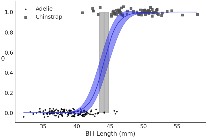
Fig. 50 拟合后的逻辑斯谛回归，显示 model_logistic_penguins_bill_length 的概率曲线、观测数据点和决策边界。仅从观测数据来看，两个物种的喙长似乎在 $45$ 毫米左右存在区分，我们的模型同样识别出围绕该值的这种区分。¶

Table 5 Logistic regression coefficients for model_logistic_penguins_bill_length.¶
	mean	sd	hdi_3%	hdi_97%
$\beta_0$	-46.052	7.073	-58.932	-34.123
$\beta_1$	1.045	0.162	0.776	1.347

现在尝试一些不同的东西，我们仍然想对企鹅进行分类，但这次使用企鹅的体重作为预测变量。代码 model_logistic_penguins_mass 显示了该模型：

Listing 35 model_logistic_penguins_mass¶

mass_obs = penguins.loc[species_filter, "body_mass_g"].values

with pm.Model() as model_logistic_penguins_mass:
    β_0 = pm.Normal("β_0", mu=0, sigma=10)
    β_1 = pm.Normal("β_1", mu=0, sigma=10)

    μ = β_0 + pm.math.dot(mass_obs, β_1)
    θ = pm.Deterministic("θ", pm.math.sigmoid(μ))
    bd = pm.Deterministic("bd", -β_0/β_1)

    yl = pm.Bernoulli("yl", p=θ, observed=species.codes)

    inf_data_logistic_penguins_mass = pm.sample(
        5000, target_accept=.9, return_inferencedata=True)

Table 6 Logistic regression coefficients for model_logistic_penguins_mass.¶
	mean	sd	hdi_3%	hdi_97%
$\beta_0$	-1.131	1.317	-3.654	1.268
$\beta_1$	0.000	0.000	0.000	0.001

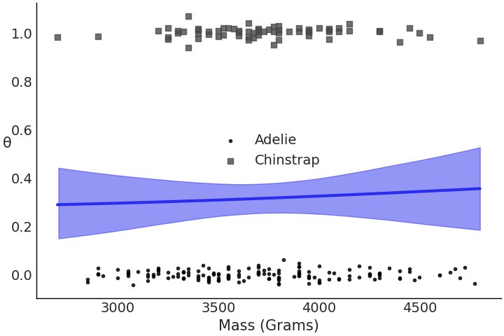
在 Table 6 表格展示的摘要信息中， $\beta_1$ 被估计为 $0$ ，表明体重预测变量中并没有足够信息来区分两个物种。这不一定是坏事，只是表明模型在两个物种的体重之间没有发现明显的差异。

一旦我们在 Fig. 51 中绘制数据和逻辑斯谛回归的拟合结果，这一点就会表现得非常明显。

Fig. 51 model_logistic_penguins_mass 的观测数据和逻辑斯谛回归图。与 Fig. 50 不同，数据看起来不可分离3。¶

我们不应该受到这种关系的缺失影响，因为有效的建模就包含一定的试错环节。这不意味着随意试错，以期能够“瞎猫碰个死耗子”，而是意味着可以使用计算工具为你提供进行下一步的线索。

现在尝试同时使用喙长度和体重，在代码 model_logistic_penguins_bill_length_mass 中创建多元逻辑斯谛回归，并在 Fig. 52 中绘制决策边界。这次图中的坐标轴有点不同， Y 轴不再是分类概率，而是企鹅的体重。这样就可以明显地看到预测变量之间的决策边界。所有这些目视检查都是有帮助的，但也是主观的。我们可以使用一些诊断工具来量化拟合程度。

Listing 36 model_logistic_penguins_bill_length_mass¶

X = penguins.loc[species_filter, ["bill_length_mm", "body_mass_g"]]

# Add a column of 1s for the intercept
X.insert(0,"Intercept", value=1)
X = X.values

with pm.Model() as model_logistic_penguins_bill_length_mass:
    β = pm.Normal("β", mu=0, sigma=20, shape=3)

    μ = pm.math.dot(X, β)

    θ = pm.Deterministic("θ", pm.math.sigmoid(μ))
    bd = pm.Deterministic("bd", -β[0]/β[2] - β[1]/β[2] * X[:,1])

    yl = pm.Bernoulli("yl", p=θ, observed=species.codes)

    inf_data_logistic_penguins_bill_length_mass = pm.sample(
        1000,
        return_inferencedata=True)

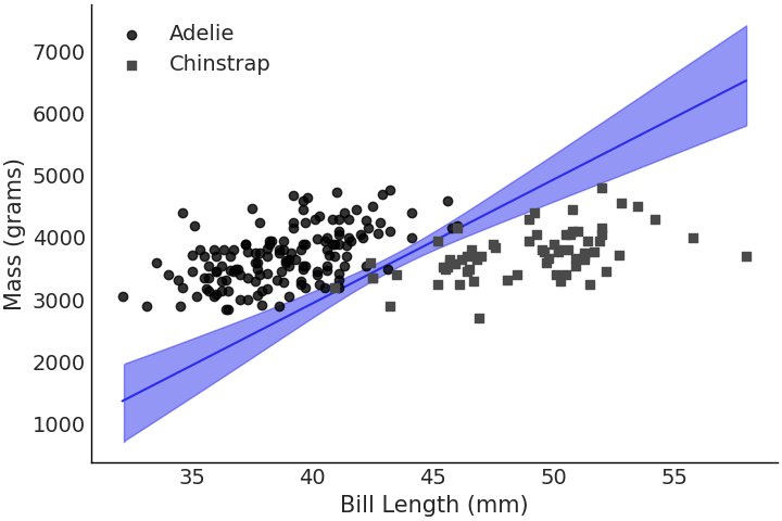
../_images/Decision_Boundary_Logistic_mass_bill_length.png

Fig. 52 针对喙长度和体重绘制的物种类别决策边界。可以看到大部分可分离性来自喙长度，尽管体重也添加了一些关于可分离性的额外信息，如线的斜率。¶

为了评估模型是否适合逻辑斯谛回归，可以使用分离图 [39]，如代码 separability_plot 和 Fig. 53 所示。分离图是一种评估二值观测数据模型校准的方法。它显示了每个类的预测排序，当两个类完美分离时，应当体现为两个不同颜色的矩形。在本示例中，可以看到我们的模型没有一个能够完美地分离两个物种，但包含喙长度的模型比仅包含体重的模型表现得更好。一般来说，完美校准不是贝叶斯分析的目标，使用分离图（以及其他校准评估方法，如 LOO-PIT）的目的是帮助我们比较模型并揭示改进它们的机会。

Listing 37 separability_plot¶

models = {"bill": inf_data_logistic_penguins_bill_length,
          "mass": inf_data_logistic_penguins_mass,
          "mass bill": inf_data_logistic_penguins_bill_length_mass}

_, axes = plt.subplots(3, 1, figsize=(12, 4), sharey=True)
for (label, model), ax in zip(models.items(), axes):
    az.plot_separation(model, "p", ax=ax, color="C4")
    ax.set_title(label)

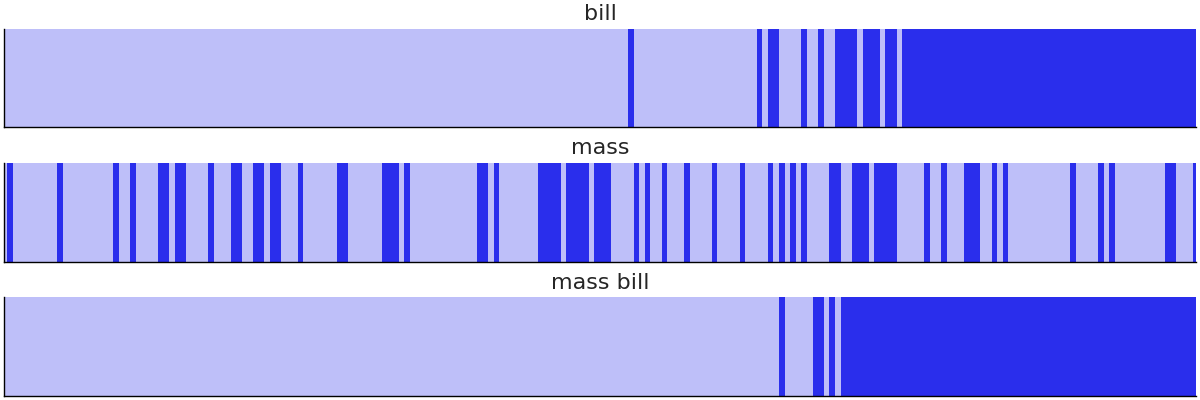
Fig. 53 三个企鹅模型的分离图。明暗值表示二分类标签。图中明显看出，仅含体重的模型在区分两个物种方面做得很差，而 单喙长度 模型和 体重-喙 模型表现更好。¶

我们还可以使用 留一法（ LOO ） 来比较刚创建的三个模型：单体重模型、单喙长度模型和代码 penguin_model_loo 和 Table 7 中的“体重+喙长度”二元预测模型。根据 LOO，单体重模型在分离物种方面表现最差，单喙长模型是中间候选模型，“体重+喙长度” 模型表现最好。上面分离图中的结果，现在得到了数值上的确认。

Listing 38 penguin_model_loo¶

az.compare({"mass":inf_data_logistic_penguins_mass,
            "bill": inf_data_logistic_penguins_bill_length,
            "mass_bill":inf_data_logistic_penguins_bill_length_mass})

Table 7 模型比较的汇总。模型按照 ELPD ( loo 列 ) 值从低到高的排序。¶
	rank	loo	p_loo	d_loo	weight	se	dse	warning	loo_scale
mass_bill	0	-11.3	1.6	0.0	1.0	3.1	0.0	True	log
bill	1	-27.0	1.7	15.6	0.0	6.2	4.9	True	log
mass	2	-135.8	2.1	124.5	0.0	5.3	5.8	True	log

3.4.3 解读对数赔率（ Log Odds ）¶

在逻辑斯谛回归中，斜率告诉你当 $x$ 增加一个单位时，增加了多少对数赔率（log odds）单位。赔率指事件发生的概率与不发生的概率之比。例如，在企鹅示例中，如果从 Adelie 种或 Chinstrap 种 企鹅中随机选择一只企鹅，那么我们选中 Adelie 种企鹅的概率将为 $0.68$，如代码 adelie_prob 所示

Listing 39 adelie_prob¶

# Class counts of each penguin species
counts = penguins["species"].value_counts()
adelie_count = counts["Adelie"],
chinstrap_count = counts["Chinstrap"]
adelie_count / (adelie_count + chinstrap_count)

array([0.68224299])

对于同一事件，赔率将是 $2.14$：

Listing 40 adelie_odds¶

adelie_count / chinstrap_count

array([2.14705882])

赔率由与概率相同的组分组成，但以一种更直接地方式，解释了一个事件发生与另一个事件发生的比率。以赔率表示，如果从 Adelie 种和 Chinstrap 种企鹅中随机采样，则根据代码 adelie_odds 计算，我们预计最终得到的 Adelie 种企鹅的赔率比 Chinstrap 种 企鹅高 $2.14$。

利用对赔率的了解，我们可以定义 logit。 logit 是赔率的自然对数，它是公式 (30) 中显示的分数。我们可以用 logit 重写公式 (29) 中的逻辑斯谛回归。

(30)¶\[\log \left(\frac{p}{1-p} \right) = \boldsymbol{X} \beta \]

该替代公式让我们可以将逻辑斯谛回归的系数解释为对数赔率的变化。此时，如果给定喙长度的变化，我们可以计算出观测到 Adelie 种 到 Chinstrap 种企鹅的概率，如代码 logistic_interpretation 所示。

像这样的转换在数学上很有趣，而且在讨论统计结果时也非常实用，我们将在 9.10 与特定受众分享结果中更深入地讨论这个主题。

Listing 41 logistic_interpretation¶

x = 45
β_0 = inf_data_logistic_penguins_bill_length.posterior["β_0"].mean().values
β_1 = inf_data_logistic_penguins_bill_length.posterior["β_1"].mean().values
bill_length = 45

val_1 = β_0 + β_1*bill_length
val_2 = β_0 + β_1*(bill_length+1)

f"""(Class Probability change from 45mm Bill Length to 46mm:
{(special.expit(val_2) -  special.expit(val_1))*100:.0f}%)"""

'Class Probability change from 45mm Bill Length to 46mm: 15%'

3.5 回归模型的先验选择¶

熟悉了广义线性模型之后，现在让我们关注一下先验及其对后验估计的影响。我们将从 [40] 中借用一个例子，特别是其中一项父母吸引力与生女孩的概率之间的关系研究[13]。在这项研究中，研究人员以五分制评估了美国青少年的吸引力。最终，这些受试者中许多人都有了孩子，其中每种吸引力类别对应的性别比例都在代码 uninformative_prior_sex_ratio 中做了计算，其结果以数据点形式显示在 Fig. 54 中。在同一个代码块中，我们还编写了一个单变量回归模型。这一次重点关注如何对先验和似然一起评估，而不是分别评估。

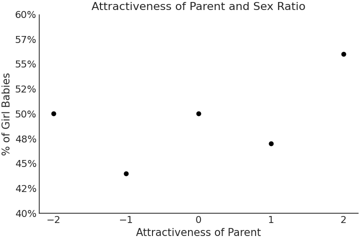
Fig. 54 父母的吸引力数据与子女的性别比例图。¶

Listing 42 uninformative_prior_sex_ratio¶

x = np.arange(-2, 3, 1)
y = np.asarray([50, 44, 50, 47, 56])

with pm.Model() as model_uninformative_prior_sex_ratio:
    σ = pm.Exponential("σ", .5)
    β_1 = pm.Normal("β_1", 0, 20)
    β_0 = pm.Normal("β_0", 50, 20)

    μ = pm.Deterministic("μ", β_0 + β_1 * x)

    ratio = pm.Normal("ratio", mu=μ, sigma=σ, observed=y)

    prior_predictive_uninformative_prior_sex_ratio = pm.sample_prior_predictive(
        samples=10000
    )
    trace_uninformative_prior_sex_ratio = pm.sample()
    inf_data_uninformative_prior_sex_ratio = az.from_PyMC3(
        trace=trace_uninformative_prior_sex_ratio,
        prior=prior_predictive_uninformative_prior_sex_ratio
    )

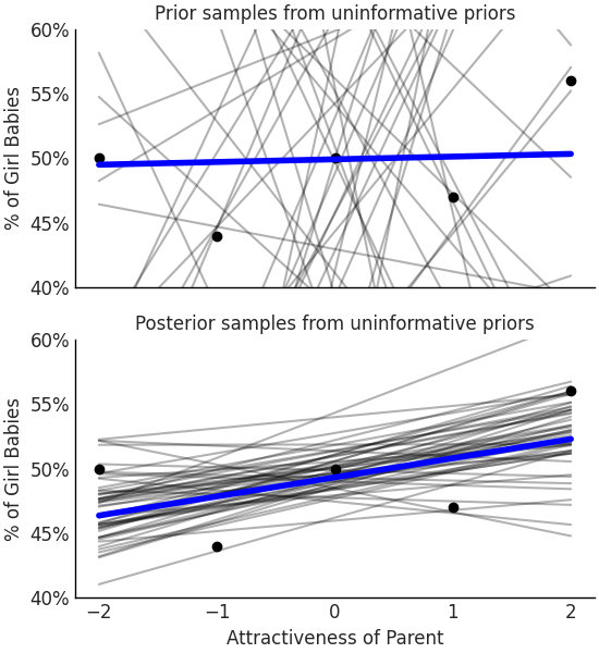
../_images/PosteriorUninformativeLinearRegression.png

Fig. 55 在采用模糊先验或宽泛先验的情况下，该模型表明，有吸引力的父母所生孩子的性别比率存在很大差异。其中一些拟合值存在高达 20% 的变化，这似乎令人难以置信，因为没有其他研究表明吸引力会对出生性别有如此大的影响。¶

名义上讲，我们将假设生男孩和生女孩的比例一样，并且吸引力对性别比例没有影响。这意味着将截距 $\beta_0$ 的先验均值设置为 $50$，将斜率 $\beta_1$ 的先验均值设置为 $0$；并且由于我们缺乏领域专业知识，因为还为两个参数都设置了比较宽泛的先验以表达这种不确定性。该先验并非一个完全无信息的先验（ 1.4 先验分布的选择方法），但它确实是一个非常宽泛的先验。

根据上述选择，我们在代码 uninformative_prior_sex_ratio) 中编写了模型、运行推断、并生成样本来估计后验分布。

根据数据和模型， $\beta_1$ 的估计均值为 $1.4$，这意味着与最具吸引力的群体相比，吸引力最小的群体的男女出生率平均相差 $7.4\%$ 。在 Fig. 55 中，如果考虑不确定性，则在将参数条件化为数据之前，从 $50$ 条可能的 “拟合线” 样本中，每单位吸引力的变化可能带来超过 $20\%$ 的男女出生比率变化。

从数学角度来看，此结果是有效的。但从常识和出生性别比来理解，此结果值得怀疑。出生时的“自然”性别比约为 “ $105$ 个男孩/$100$ 个女孩” ( 大约 $103$ 到 $107$ 个男孩 )，这意味着出生时的性别比为 $48.5%$ ，标准差为 $0.5$。此外，即便与人类生物学存在内在联系因素，也不会对出生率影响到这种大程度，这主观上削弱了吸引力应该具有此影响程度的信念。鉴于此信息，两组之间 $8%$ 的变化将需要特殊的观测。

让我们再次运行模型，但这次使用代码 informative_prior_sex_ratio 中的信息性先验。抽取后验样本，会发现系数的分布非常集中，并且在考虑可能的比率时，抽取的后验预测直线会落入了更合理的范围内。

Listing 43 informative_prior_sex_ratio¶

with pm.Model() as model_informative_prior_sex_ratio:
    σ = pm.Exponential("σ", .5)

    # Note the now more informative priors
    β_1 = pm.Normal("β_1", 0, .5)
    β_0 = pm.Normal("β_0", 48.5, .5)

    μ = pm.Deterministic("μ", β_0 + β_1 * x)
    ratio = pm.Normal("ratio", mu=μ, sigma=σ, observed=y)

    prior_predictive_informative_prior_sex_ratio = pm.sample_prior_predictive(
        samples=10000
    )
    trace_informative_prior_sex_ratio = pm.sample()
    inf_data_informative_prior_sex_ratio = az.from_PyMC3(
        trace=trace_informative_prior_sex_ratio,
        prior=prior_predictive_informative_prior_sex_ratio)

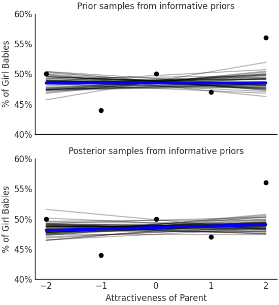
../_images/PosteriorInformativeLinearRegression.png

Fig. 56 根据其他论文和专家知识优化后的先验，平均后验在吸引力比率上几乎没有变化，这表明如果认为父母吸引力对出生率有影响，则应该收集更多数据来展示这种影响。¶

这次我们看到吸引力对性别的影响几乎可以忽略不计，根本没有足够信息来影响后验。正如在 1.4 先验分布的选择方法节中提到的，选择先验既是负担也是祝福。无论你认为是哪一种，重要的是使用这种统计工具并做出可解释和有原则的选择。

习题¶

E1. Comparisons are part of everyday life. What is something you compare on a daily basis and answer the following question:

What is the numerical quantification you use for comparison?
How do you decide on the logical groupings for observations? For example in the penguin model we use species or sex
What point estimate would you use to compare them?

E2. Referring to Model penguin_mass complete the following tasks.

Compute the values of Monte Carlo Standard Error Mean using az.summary. Given the computed values which of the following reported values of $\mu$ would not be well supported as a point estimate? 3707.235, 3707.2, or 3707.
Plot the ESS and MCSE per quantiles and describe the results.
Resample the model using a low number of draws until you get bad values of $\hat R$, and ESS
Report the HDI $50\%$ numerically and using az.plot_posterior

E3. In your own words explain how regression can be used to do the following:

Covariate estimation
Prediction
Counterfactual analysis

Explain how they are different, the steps to perform each, and situations where they would be useful. Use the penguin example or come up with your own.

E4. In Code Block flipper_centering and Code Block tfp_penguins_centered_predictor we centered the flipper length covariate. Refit the model, but instead of centering, subtract the minimum observed flipped length. Compare the posterior estimates of the slope and intercept parameters of the centered model. What is different, what is the same. How does the interpretation of this model change when compared to the centered model?

E5. Translate the following primitives from PYMC3 to TFP. Assume the model name is pymc_model

pm.StudentT("x", 0, 10, 20)
pm.sample(chains=2)

Hint: write the model and inference first in PYMC3, and find the similar primitives in TFP using the code shown in this chapter.

E6. PYMC3 and TFP use different argument names for their distribution parameterizations. For example in PYMC3 the Uniform Distribution is parameterized as pm.Uniform.dist(lower=, upper=) whereas in TFP it is tfd.Uniform(low=, high=). Use the online documentation to identify the difference in argument names for the following distributions.

Normal
Poisson
Beta
Binomial
Gumbel

E7. A common modeling technique for parameterizing Bayesian multiple regressions is to assign a wide prior to the intercept, and assign more informative prior to the slope coefficients.

Try modifying the model_logistic_penguins_bill_length_mass model in Code Block model_logistic_penguins_bill_length_mass.

Do you get better inference results? Note that there are divergence with the original parameterization.

E8. In linear regression models we have two terms. The mean linear function and the noise term. Write down these two terms in mathematical notation, referring to the equations in this chapter for guidance. Explain in your own words what the purpose of these two parts of regression are. In particular why are they useful when there is random noise in any part of the data generating or data collection process.

E9. Simulate the data using the formula y = 10 + 2x + $\mathcal{N}(0, 5)$ with integer covariate x generated np.linspace(-10, 20, 100). Fit a linear model of the form $b_0 + b_1*X + \sigma$. Use a Normal distribution for the likelihood and covariate priors and a Half Student’s T prior for the noise term as needed. Recover the parameters verifying your results using both a posterior plot and a forest plot.

E10. Generate diagnostics for the model in Code Block non_centered_regression to verify the results shown in the chapter can be trusted. Use a combination of visual and numerical diagnostics.

E11. Refit the model in Code Block non_centered_regression on Gentoo penguins and Chinstrap penguins. How are the posteriors different from each other? How are they different from the Adelie posterior estimation? What inferences can you make about the relationship between flipper length and mass for these other species of penguins? What does the change in $\sigma$ tell you about the ability of flipper length to estimate mass?

M12. Using the model in Code Block tfp_flipper_bill_sex_counterfactuals run a counterfactual analysis for female penguin flipper length with mean flipper length and a bill length of 20mm. Plot a kernel density estimate of the posterior predictive samples.

M13. Duplicate the flipper length covariate in Code Block non_centered_regression by adding a $\beta_2$ coefficient and rerun the model. What do diagnostics such as ESS and rhat indicate about this model with a duplicated coefficient?

M14. Translate the PYMC3 model in Code Block non_centered_regression into Tensorflow Probability. List three of the syntax differences.

M15. Translate the TFP model in Code Block tfp_penguins_centered_predictor into PYMC3. List three of the syntax differences.

M16. Use a logistic regression with increasing number of covariates to reproduce the prior predictive distributions in Fig. 14.

Explain why its the case that a logistic regression with many covariates generate a prior response with extreme values.

H17. Translate the PYMC3 model in Code Block model_logistic_penguins_bill_length_mass into TFP to classify Adelie and Chinstrap penguins. Reuse the same model to classify Chinstrap and Gentoo penguins. Compare the coefficients, how do they differ?

H18. In Code Block penguin_mass our model allowed for negative values mass. Change the model so negative values are no longer possible. Run a prior predictive check to verify that your change was effective. Perform MCMC sampling and plot the posterior. Has the posterior changed from the original model? Given the results why would you choose one model over the other and why?

H19. The Palmer Penguin dataset includes additional data for the observed penguins such as island and bill depth. Include these covariates into the linear regression model defined in Code Block non_centered_regression in two parts, first adding bill depth, and then adding the island covariates.

Do these covariates help estimate Adelie mass more precisely? Justify your answer using the parameter estimates and model comparison tools.

H20. Similar the exercise 2H19, see if adding bill depth or island covariates to the penguin logistic regression help classify Adelie and Gentoo penguins more precisely. Justify if the additional covariates helped using the numerical and visual tools shown in this chapter.

参考文献¶

Nature can be hard to grasp with simple statements.

1: You can find more information in the TensorFlow tutorials and documentations. For example, https://www.tensorflow.org/probability/examples/JointDistributionAutoBatched_A_Gentle_Tutorial and https://www.tensorflow.org/probability/examples/Modeling_with_JointDistribution.
2: tfd.Sample and tfd.Independent are distribution constructors that takes other distributions as input and return a new distribution. There are other meta distribution but with different purposes like tfd.Mixture, tfd.TransformedDistribution, and tfd.JointDistribution. A more comprehensive introduction to tfp.distributions can be found in https://www.tensorflow.org/probability/examples/TensorFlow_Distributions_Tutorial
3: https://mc-stan.org/docs/2_23/reference-manual/hmc-algorithm-parameters.html#automatic-parameter-tuning
4: If wanted exactly the same model we could specify the priors in Bambi, not shown here. For our purposes however, the models are “close enough”.
5: You can also parse the design matrix differently so that covariates represents the contrast between 2 categories within a column.
6: Maybe because collecting more data is expensive or difficult or even impossible
7: Unless we are talking about large systems like rain forests, where the presence of plants actually have an impact in the weather.
8: Traditionally people aPPLy functions like $\phi$ to the left side of Equation (28), and call them link functions. We instead prefer to aPPLy them to the right-hand side and then to avoid confusion we use term inverse link function.
9: Usually in the traditional Generalized Linear Models Literature, the likelihood of the observation need to be from the Exponential family, but being Bayesian we are actually not restricted by that and can use any likelihood that can be parameterized by the expected value.

Bayesian Modeling and Computation in Python

第三章：线性模型与概率编程语言

Contents