第十一章：附加主题¶

本章与其他章节不同，它不是关于任何特定主题的。相反，它是不同主题的集合，通过补充其他章节中讨论的主题，为本书的其余部分提供支撑。这些主题适用于有兴趣深入了解每种理论和方法的读者。就写作风格而言，本章将比其他章节更具理论性和抽象性。

11.1 概率背景¶

西班牙语单词 azahar 和 azar 含义不同并非纯属运气，因为它们都来自于阿拉伯语 1。从远古时代开始至今，一些机会游戏会使用具有两个面的骨头，这种骨头类似于硬币或双面骰子。为了更容易区分一侧和另一侧，其中至少一侧有明显的标记，古代阿拉伯人常用一朵花做标记。随着时间推移，西班牙语逐步采用了 azahar 一词来表示某些花，而用 azar 表示随机性。

概率论发展的动机之一可以追溯到理解机会游戏，并试图在此过程中发点小财。因此，让我们简要从六面骰子（ Die With Six Faces ）开始，介绍概率论中一些核心概念2。每次掷骰子时，只能获得一个从 \(1\) 到 \(6\) 的整数，而且他们之间相互没有依从喜好。使用 Python，可以通过以下方式编写这样的骰子游戏：

Listing 161 die¶

def die():
    outcomes = [1, 2, 3, 4, 5, 6]
    return np.random.choice(outcomes)

假设我们怀疑骰子有偏差，如何才能评估这种可能性？回答此问题的科学方法是收集并分析数据。使用 Python，我们可以模拟代码 experiment 中的数据收集过程。

Listing 162 实验¶

def experiment(N=10):
    sample = [die() for i in range(N)]

    for i in range(1, 7):
        print(f"{i}: {sample.count(i)/N:.2g}")

experiment()

0
0.1
0.4
0.1
0.4
0

第一列中的数字是可能的结果。第二列对应于每个数字出现的频率。频率是每个可能结果出现的次数除以掷骰子的总次数（即 “N” ）。

在这个例子中至少有两点需要注意。

首先如果执行 experiment() 几次，我们每次都会得到不同的结果。这正是在机会游戏中使用骰子的原因，每次掷骰子都会得到一个我们无法预测的数字。

其次，即使多次掷同一个骰子，预测每个结果的能力也并没有提高。

尽管如此，数据收集和分析还是可以帮助我们估计结果的频率列表，事实上，随着 “N” 值的增加，这种能力会有所提高。运行实验 N=10000 次，你会看到获得的频率约为 \(0.17\) 。如果骰子上的每个数字有同样的机会，该结果也表明 \(0.17 \approx \frac{1}{6}\) 正是我们所预期的。

上述两点观测不仅限于骰子和机会游戏。

如果每天称体重，我们会得到不同的值，因为体重与吃的食物量、喝的水、上厕所的次数、秤的精度、穿的衣服和许多其他因素有关。因此，单次测量可能无法代表我们的体重，但重要的是，数据测量和/或收集伴随着不确定性。

统计学基本上是关于如何处理实际问题中的不确定性的领域，概率论是统计学的理论支柱之一。概率论帮助我们将讨论的内容形式化，就像刚刚讨论的那样，并将其扩展到骰子之外。这样我们就可以更好地提出和解答与预期结果相关的问题，例如当增加实验次数时会发生什么？什么事件比另一个事件更有机会？

11.1.1 概率¶

概率是一种允许我们量化不确定性的理论数学工具。像其他数学对象和理论一样，它们完全可以从纯数学角度来证明。然而，从实践角度来看，我们可以证明概率是通过进行实验、收集观测数据甚至在进行计算模拟时自然产生的。为简单起见，我们将讨论实验，因为我们在非常广泛的意义上在使用该术语。

我们可以用数学集合来思考概率。 样本空间 \(\mathcal{X}\) 是来自实验的所有可能事件的集合。事件 \(A\) 是 \(\mathcal{X}\) 的子集。在我们进行实验时，称 \(A\) 事件发生，并得到集合 \(A\) 作为结果。对于典型的六面骰子，可以写为：

(85)¶\[\mathcal{X} = \{1, 2, 3, 4, 5, 6\}\]

我们可以将事件 \(A\) 定义为 \(\mathcal{X}\) 的任何子集，例如，得到偶数 \(A = \{2, 4, 6\}\)。我们将概率与事件联系起来，如果想表示事件 \(A\) 的概率，可以写成 \(P(A=\{2, 4, 6\})\) 或更简洁的 \(P(A)\) 。概率函数 \(P\) 将事件 \(A\) 作为输入并返回 \(P(A)\) 。概率 \(P(A)\) 可以取区间 \([0,1]\) 中的任何数字。如果事件从未发生，则该事件的概率为 \(0\)，例如 \(P(A=-1)=0\) ；如果事件总是发生，则概率为 \(1\) ，例如 \(P(A=\{1, 2,3,4,5,6\})=1\) 。如果事件不能一起发生，我们就称事件是互斥的，例如，如果事件 \(A_1\) 代表奇数， \(A_2\) 代表偶数数字，那么掷骰子同时得到 \(A_1\) 和 \(A_2\) 的概率为 \(0\) 。如果事件 \(A_1, A_2, \cdots A_n\) 是互斥的，意味着这些事件不能同时发生，那么 \(\sum_i^n P(A_i) = 1\) 。继续 \(A_1\) 表示奇数、 \(A_2\) 表示偶数的示例，掷骰子的结果为 \(A_1\) 或 \(A_2\) 的概率为 \(1\) 。满足此性质的任何函数都是有效的概率函数。我们可以将概率视为分配给可能事件的正守恒量 3 。

正如刚刚看到的，概率有一个明确的数学定义。如何解释概率有着不同的故事，也有着不同的思想流派。作为贝叶斯主义者，我们倾向于将概率解释为不确定性的程度。例如，对于一个公平的骰子，掷骰子时得到奇数的概率是 \(50\%\) ，这意味着我们有一半把握会得到一个奇数。或者可以将这个数字解释为，如果无限次掷骰子，有一半的时间会得到奇数，一半的时间会得到偶数，而这是频率主义者的解释。如果你不想无限次掷骰子，也可以多次掷骰子，然后获得大约一半的几率。这实际上就是在代码 experiment 中做的。最后，我们注意到对于公平骰子，期望得到任何单个数字的概率为 \(\frac{1}{6}\)，但对于非公平骰子，此概率可能有所不同，而等概率结果只是一个特例。

如果概率反映了不确定性，那么提出 “火星的质量是 \(6.39 \times 10^{23}\) 公斤的概率是多少？”，或者“赫尔辛基 \(5\) 月 \(1\) 日下雨的概率是多少？”，或者“未来三年资本主义被其他社会经济制度取代的概率是多少？” 等问题，都是非常自然的。我们说概率的定义是认知层面的，因为它不是一个关于真实世界的属性，而是一个关于我们对世界认知的属性。我们收集并分析数据，因为我们认为根据外部信息，我们能够更新内心里的知识状态。

我们注意到现实世界中可能发生的事情取决于实验的所有细节，包括我们无法控制或不知道的那些。而样本空间是我们隐式或显式定义的数学对象。例如，通过将骰子的样本空间定义为方程 (85)，我们排除了骰子落在边缘的可能性，虽然这实际上在非平面中滚动骰子时有可能发生。

我们必须意识到：包含所有数学概念的柏拉图思想世界与现实世界是不同的，在统计建模时，我们需要不断在这两个世界之间来回切换。

11.1.2 条件概率¶

给定两个事件 \(A\) 和 \(B\) 且 \(P(B) > 0\)，给定 \(B\) 时事件 \(A\) 发生的概率，被记为 \(P(A \mid B)\) ，定义为：

\[P(A \mid B) = \frac{P(A, B)}{P(B)}\]

\(P(A, B)\) 是事件 \(A\) 和 \(B\) 同时发生的概率，通常也记为 \(P(A \cap B)\)（符号 \(\cap\) 表示集合的交集），即事件 \(A\) 和事件 \(B\) 同时发生的概率。

\(P(A \mid B)\) 被称为条件概率，它是指在 \(B\) 已经发生的条件下，事件 \(A\) 发生的概率。例如，“人行道潮湿的概率” 与 “在下雨的情况下人行道潮湿的概率” 是完全不同的。

条件概率可以看作是样本空间的缩减或限制。 Fig. 169 展示了从左图的样本空间 \(\mathcal{X}\) 中的事件 \(A\) 和 \(B\) ，到右图中将 \(B\) 作为样本空间而 \(A\) 为其子集。当我们说 \(B\) 已经发生，不一定是在谈论过去发生的事情，它只是 “一旦我们以 \(B\) 为条件” 或 “一旦我们将样本空间限制为与证据 \(B\) 一致” 的通俗说法。

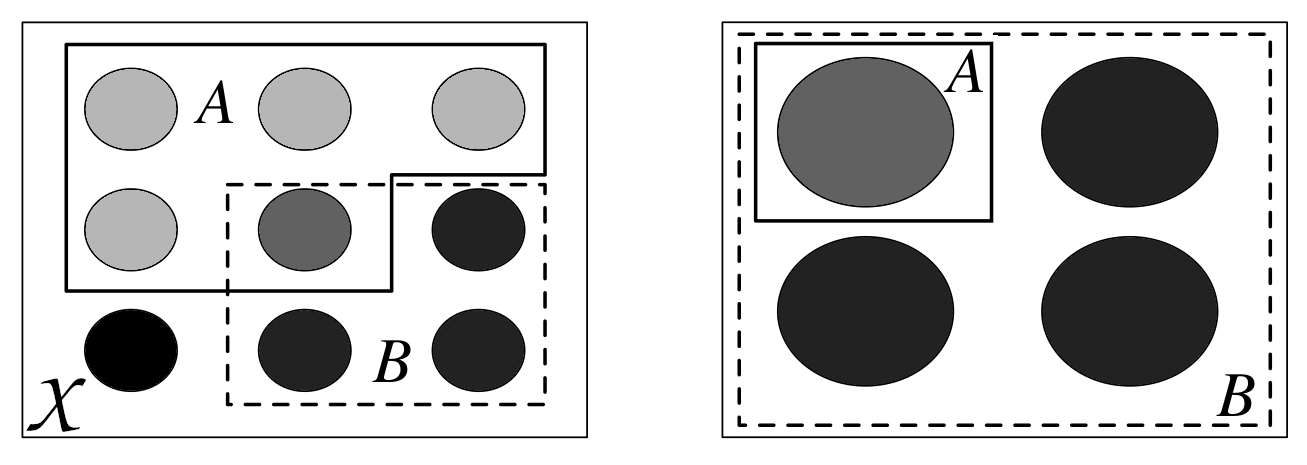
Fig. 169 条件化就是重新定义样本空间。左图为样本空间 \(\mathcal{X}\)，每个圆圈代表一个可能的结果。其中有 \(A\) 和 \(B\) 两个事件。右图代表 \(P(A \mid B)\) ，一旦知道 \(B\) ，我们就可以排除所有不在 \(B\) 中的事件。该图改编自《 Introduction to Probability 》 [5]。¶

条件概率是统计学的核心，是思考如何根据新数据更新我们对事件的知识的核心。所有的概率相对于某些假设或模型都是有条件的。从来不存在不包含上下文语境的概率，即便我们并没有明确地把这个意思表达出来。

11.1.3 概率分布¶

我们可能更感兴趣的是找出骰子上所有数字的概率列表，而不是计算掷骰子时获得数字 5 的概率。一旦计算出这个列表，我们就可以显示它或使用它来计算其他数量，比如得到数字 5 的概率，或者得到等于或大于 5 的数字的概率。这个 list 的正式名称是 probability 分配。

使用 Code Block experiment 我们得到了一个骰子的经验概率分布，即从数据中计算出来的分布。但也有理论分布，它们在统计学中很重要，因为它们允许构建概率模型。

理论概率分布具有精确的数学公式，类似于圆具有精确的数学定义。

圆是平面上与另一个称为中心的点等距的点的几何空间。给定参数半径，完美定义了一个圆 4。我们可以说不存在单个圆周，而是一个圆周族，其中每个成员与其他成员的区别仅在于参数 radius 的值，因为一旦还定义了此参数，则定义了圆周。

类似地，概率分布也出现在家族中，其成员完全由一个或多个参数定义。通常使用希腊字母来编写参数名称，尽管情况并非总是如此。 Fig. 170 是此类分布系列的一个示例，我们可以用它来表示已加载的骰子。我们可以看到这个概率分布是如何由两个参数 \(\alpha\) 和 \(\beta\) 控制的。如果我们改变分布的形状，我们可以使其平坦或集中在一侧，将大部分质量推向极端，或将质量集中在中间。由于圆周半径被限制为正，分布的参数也有限制，实际上\(\alpha\)和\(\beta\)必须都是正的。

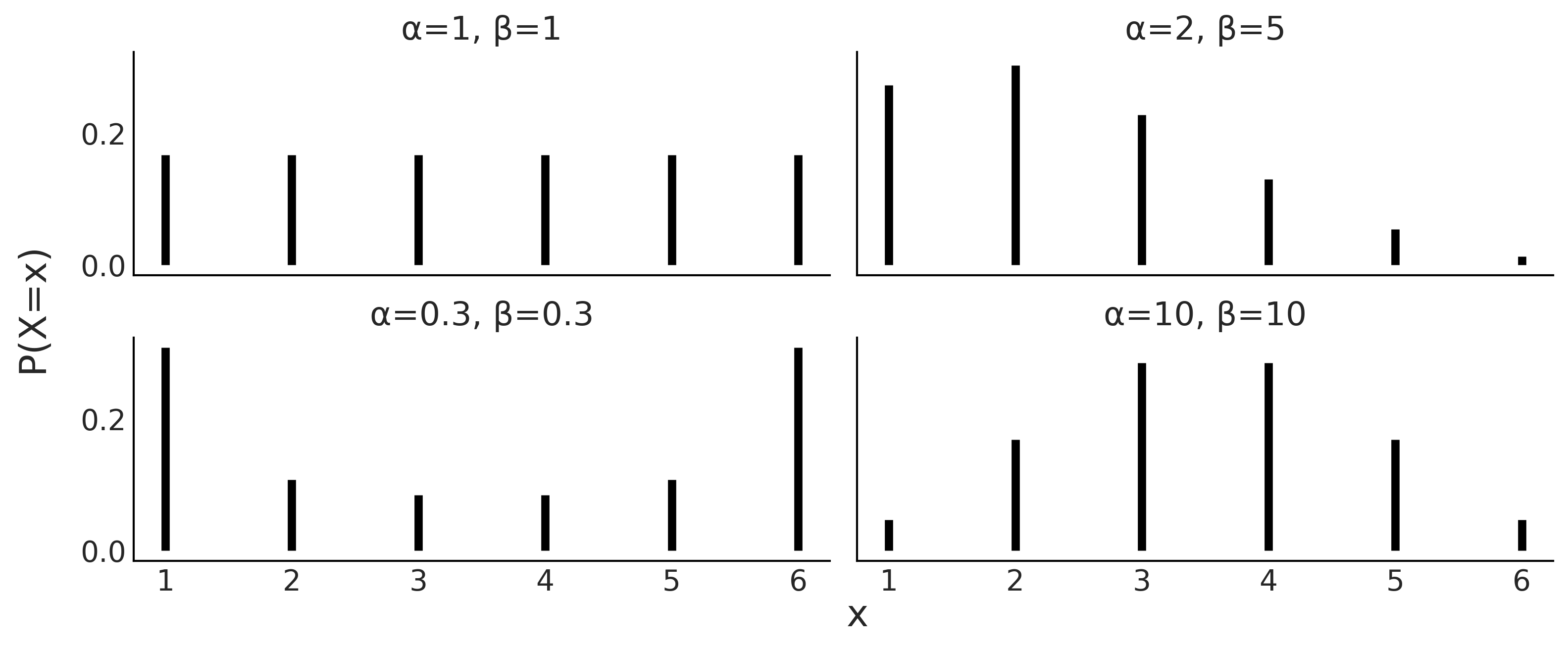
Fig. 170 具有参数 \(\alpha\) 和 \(\beta\) 的离散分布族的四个成员。条形的高度代表每个 \(x\) 值的概率。未绘制的 \(x\) 的值的概率为 0，因为它们不受分布的支持。¶

11.1.4 离散型随机变量及其分布¶

A random variable is a function that maps the sample space into the real numbers \(\mathbb{R}\). Continuing with the die example if the events of interest were the number of the die, the mapping is very simple, we associate \(\LARGE \unicode{x2680}\) with the number 1, \(\LARGE \unicode{x2681}\) with 2, etc.

With two dice we could have an \(S\) random variable as the sum of the outcomes of both dice. Thus the domain of the random variable \(S\) is \(\{2, 3, 4, 5, 6, 7, 8, 9, 10, 11, 12\}\), and if both dice are fair then their probability distribution is depicted in Fig. 171.

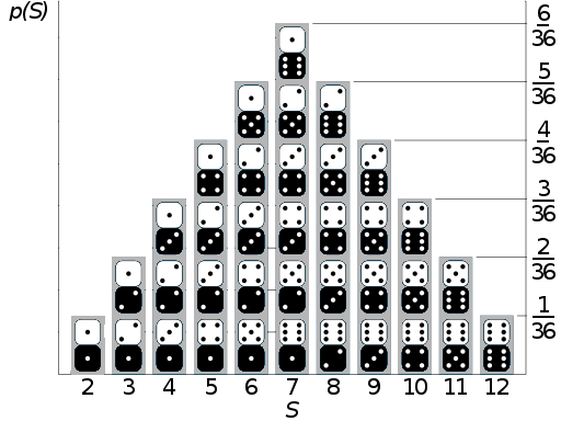
Fig. 171 If the sample space is the set of possible numbers rolled on two dice, and the random variable of interest is the sum \(S\) of the numbers on the two dice, then \(S\) is a discrete random variable whose distribution is described in this figure with the probability of each outcome represented as the height of the columns. This figure has been adapted from https://commons.wikimedia.org/wiki/File:Dice_Distribution_(bar).svg¶

We could also define another random variable \(C\) with sample space \(\{\text{red}, \text{green}, \text{blue}\}\). We could map the sample space to \(\mathbb{R}\) in the following way:

\[\begin{split}\begin{aligned} C(\text{red})\; = 0 \\ C(\text{green}) = 1 \\ C(\text{blue})\, = 2\end{aligned}\end{split}\]

This encoding is useful, because performing math with numbers is easier than with strings regardless of whether we are using analog computation on “pen and paper” or digital computation with a computer.

As we said a random variable is a function, and given that the mapping between the sample space and \(\mathbb{R}\) is deterministic it is not immediately clear where the randomness in a random variable comes from.

We say a variable is random in the sense that if we perform an experiment, i.e. we ask the variable for a value like we did in Code Block die and experiment we will get a different number each time without the succession of outcomes following a deterministic pattern. For example, if we ask for the value of random variable \(C\) 3 times in a row we may get red, red, blue or maybe blue, green, blue, etc.

A random variable \(X\) is said to be discrete if there is a finite list of values \(a_1, a_2, \dots, a_n\) or an infinite list of values \(a_1, a_2, \dots\) such that the total probability is \(\sum_j P(X=a_j) = 1\). If \(X\) is a discrete random variable then a finite or countably infinite set of values \(x\) such that \(P(X = x) > 0\) is called the support of \(X\).

As we said before we can think of a probability distribution as a list associating a probability with each event. Additionally a random variable has a probability distribution associated to it. In the particular case of discrete random variables the probability distribution is also called a Probability Mass Function (PMF). It is important to note that the PMF is a function that returns probabilities.

The PMF of \(X\) is the function \(P(X=x)\) for \(x \in \mathbb{R}\). For a PMF to be valid, it must be non-negative and sum to 1, i.e. all its values should be non-negative and the sum over all its domain should be 1.

It is important to remark that the term random in random variable does not implies that any value is allowed, only those in the sample space.

For example, we can not get the value orange from \(C\), nor the value 13 from \(S\). Another common source of confusion is that the term random implies equal probability, but that is not true, the probability of each event is given by the PMF, for example, we may have \(P(C=\text{red}) = \frac{1}{2}, P(C=\text{green}) = \frac{1}{4}, P(C=\text{blue}) = \frac{1}{4}\).

The equiprobability is just a special case.

We can also define a discrete random variable using a cumulative distribution function (CDF). The CDF of a random variable \(X\) is the function \(F_X\) given by \(F_X(x) = P(X \le x)\). For a CDF to be valid, it must be monotonically increasing 5, right-continuous 6, converge to 0 as \(x\) approaches to \(- \infty\), and converge to 1 as \(x\) approaches \(\infty\).

In principle, nothing prevents us from defining our own probability distribution. But there are many already defined distributions that are so commonly used, they have their own names. It is a good idea to become familiar with them as they appear quite often. If you check the models defined in this book you will see that most of them use combinations of predefined probability distributions and only a few examples used custom defined distribution. For example, in Section 8.6 移动平均模型的近似 Code Block MA2_abc we used a Uniform distribution and two potentials to define a 2D triangular distribution.

Figures Fig. 172, Fig. 173, and Fig. 174, are example of some common discrete distribution represented with their PMF and CDF. On the left we have the PMFs, the height of the bars represents the probability of each \(x\). On the right we have the CDF, here the jump between two horizontal lines at a value of \(x\) represents the probability of \(x\). The figure also includes the values of the mean and standard deviation of the distributions, is important to remark that these values are properties of the distributions, like the length of a circumference, and not something that we compute from a finite sample (see Section 11.1.8 期望 for details).

Another way to describe random variables is to use stories. A story for \(X\) describes an experiment that could give rise to a random variable with the same distribution as \(X\). Stories are not formal devices, but they are useful anyway. Stories have helped humans to make sense of their surrounding for millennia and they continue to be useful today, even in statistics. In the book Introduction to Probability [5] Joseph K. Blitzstein and Jessica Hwang make extensive use of this device. They even use story proofs extensively, these are similar to mathematical proof but they can be more intuitive. Stories are also very useful devices to create statistical models, you can think about how the data may have been generated, and then try to write that down in statistical notation and/or code. We do this, for example, in Chapter [9]](chap9) with our flight delay example.

( 1 ) 离散型均匀分布¶

This distribution assigns equal probability to a finite set of consecutive integers from interval a to b inclusive. Its PMF is:

(86)¶\[P(X = x) = {\frac {1}{b - a + 1}} = \frac{1}{n}\]

for values of \(x\) in the interval \([a, b]\), otherwise \(P(X = x) = 0\), where \(n=b-a+1\) is the total number values that \(x\) can take.

We can use this distribution to model, for example, a fair die. Code Block scipy_unif shows how we can use Scipy to define a distribution and then compute useful quantities such as the PMF, CDF, and moments (see Section 11.1.8 期望).

Listing 163 scipy_unif¶

a = 1
b = 6
rv = stats.randint(a, b+1)
x = np.arange(1, b+1)

x_pmf = rv.pmf(x)  # evaluate the pmf at the x values
x_cdf = rv.cdf(x)  # evaluate the cdf at the x values
mean, variance = rv.stats(moments="mv")

Using Code Block scipy_unif plus a few lines of Matplotlib we generate Fig. 172. On the left panel we have the PMF where the height of each point indicates the probability of each event, we use points and dotted lines to highlight that the distribution is discrete. On the right we have the CDF, the height of the jump at each value of \(x\) indicates the probability of that value.

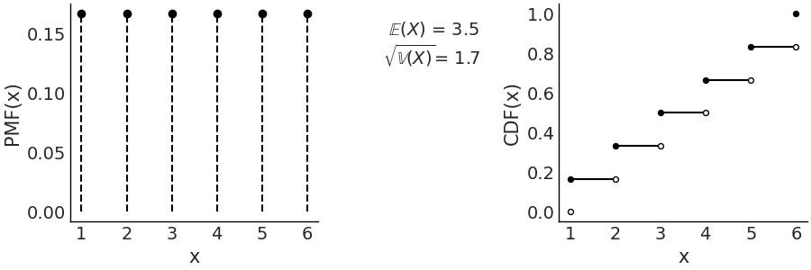
Fig. 172 Discrete Uniform with parameters (1, 6). On the left the PMF. The height of the lines represents the probabilities for each value of \(x\). On the right the CDF. The height of the jump at each value of \(x\) represent its probability. Values outside of the support of the distribution are not represented. The filled dots represent the inclusion of the CDF value at a particular \(x\) value, the open dots reflect the exclusion.¶

In this specific example the discrete Uniform distribution is defined on the interval \([1, 6]\). Therefore, all values less than 1 and greater than 6 have probability 0. Being a Uniform distribution, all the points have the same height and that height is \(\frac{1}{6}\). There are two parameters of the Uniform discrete distribution, the lower limit \(a\) and upper limit \(b\).

As we already mentioned in this chapter if we change the parameters of a distribution the particular shape of the distribution will change (try for example, replacing stats.randint(1, 7) in Code Block scipy_unif with stats.randint(1, 4). That is why we usually talk about family of distributions, each member of that family is a distribution with a particular and valid combination of parameters. Equation (86) defines the family of discrete Uniform distributions as long as \(a < b\) and both \(a\) and \(b\) are integers.

When using probability distributions to create statistical applied models it is common to link the parameters with quantities that make physical sense. For example, in a 6 sided die it makes sense that \(a=1\) and \(b=6\). In probability we generally know the values of these parameters while in statistics we generally do not know these values and we use data to infer them.

( 2 ) 二项分布¶

A Bernoulli trial is an experiment with only two possible outcomes yes/no (success/failure, happy/sad, ill/healthy, etc). Suppose we perform \(n\) independent 7 Bernoulli trials, each with the same success probability \(p\) and let us call \(X\) the number of success. Then the distribution of \(X\) is called the Binomial distribution with parameters \(n\) and \(p\), where \(n\) is a positive integer and \(p \in [0, 1]\). Using statistical notation we can write \(X \sim Bin(n, p)\) to mean that \(X\) has the Binomial distribution with parameters \(n\) and \(p\), with the PMF being:

\[P(X = x) = \frac{n!}{x!(n-x)!}p^x(1-p)^{n-x}\]

The term \(p^x(1-p)^{n-x}\) counts the number of \(x\) success in \(n\) trials. This term only considers the total number of success but not the precise sequence, for example, \((0,1)\) is the same as \((1,0)\), as both have one success in two trials. The first term is known as Binomial Coefficient and computes all the possible combinations of \(x\) elements taken from a set of \(n\) elements.

The Binomial PMFs are often written omitting the values that return 0, that is the values outside of the support. Nevertheless it is important to be sure what the support of a random variable is in order to avoid mistakes. A good practice is to check that PMFs are valid, and this is essential if we are proposing a new PMFs instead of using one off the shelf.

When \(n=1\) the Binomial distribution is also known as the Bernoulli distribution. Many distributions are special cases of other distributions or can be obtained somehow from other distributions.

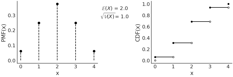
Fig. 173 \(\text{Bin}(n=4, p=0.5)\) On the left the PMF. The height of the lines represents the probabilities for each value of \(x\). On the right the CDF. The height of the jump at each value of \(x\) represent its probability. Values outside of the support of the distribution are not represented.¶

( 3 ) 泊松分布¶

This distribution expresses the probability that \(x\) events happen during a fixed time interval (or space interval) if these events occur with an average rate \(\mu\) and independently from each other. It is generally used when there are a large number of trials, each with a small probability of success. For example

Radioactive decay, the number of atoms in a given material is huge, the actual number that undergo nuclear fission is low compared to the total number of atoms.
The daily number of car accidents in a city. Even when we may consider this number to be high relative to what we would prefer, it is low in the sense that every maneuver that the driver performs, including turns, stopping at lights, and parking, is an independent trial where an accident could occur.

The PMF of a Poisson is defined as:

(87)¶\[P(X = x) = \frac{\mu^{x} e^{-\mu}}{x!}, x = 0, 1, 2, \dots\]

Notice that the support of this PMF are all the natural numbers, which is an infinite set. So we have to be careful with our list of probabilities analogy, as summing an infinite series can be tricky. In fact Equation (87) is a valid PMF because of the Taylor series \(\sum_0^{\infty} \frac{\mu^{x}}{x!} = e^{\mu}\)

Both the mean and variance of the Poisson distribution are defined by \(\mu\). As \(\mu\) increases, the Poisson distribution approximates to a Normal distribution, although the latter is continuous and the Poisson is discrete. The Poisson distribution is also closely related to the Binomial distribution. A Binomial distribution can be approximated with a Poisson, when \(n >> p\) 8, that is, when the probability of success (\(p\)) is low compared with the number o trials (\(n\)) then \(\text{Pois}(\mu=np) \approx \text{Bin}(n, p)\). For this reason the Poisson distribution is also known as the law of small numbers or the law of rare events. As we previously mentioned this does not mean that \(\mu\) has to be small, but instead that \(p\) is low with respect to \(n\).

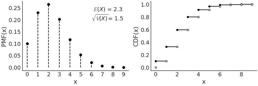
Fig. 174 \(\text{Pois}(2.3)\) On the left the PMF. The height of the lines represents the probabilities for each value of \(x\). On the right the CDF. The height of the jump at each value of \(x\) represent its probability. Values outside of the support of the distribution are not represented.¶

11.1.5 连续型随机变量及其分布¶

So far we have seen discrete random variables. There is another type of random variable that is widely used called continuous random variables, whose support takes values in \(\mathbb {R}\). The most important difference between discrete and continuous random variables is that the latter can take on any \(x\) value in an interval, although the probability of any \(x\) value is exactly 0. Introduced this way you may think that these are the most useless probability distributions ever.

But that is not the case, the actual problem is that our analogy of treating a probability distribution as a finite list is a very limited analogy and it fails badly with continuous random variables 9.

In Figures Fig. 172, Fig. 173, and Fig. 174, to represent PMFs (discrete variables), we used the height of the lines to represent the probability of each event. If we add the heights we always get 1, that is, the total sum of the probabilities. In a continuous distribution we do not have lines but rather we have a continuous curve, the height of that curve is not a probability but a probability density and instead of of a PMF we use a Probability Density Function (PDF). One important difference is that height of \(\text{PDF}(x)\) can be larger than 1, as is not the probability value but a probability density. To obtain a probability from a PDF instead we must integrate over some interval:

\[P(a < X < b) = \int_a^b pdf(x) dx\]

Thus, we can say that the area below the curve of the PDF (and not the height as in the PMF) gives us a probability, the total area under the curve, i.e. evaluated over the entire support of the PDF, must integrate to 1. Notice that if we want to find out how much more likely the value \(x_1\) is compared to \(x_2\) we can just compute \(\frac{pdf(x_1)}{pdf(x_2)}\).

In many texts, including this one, it is common to use the symbol \(p\) to talk about the \(pmf\) or \(pdf\). This is done in favour of generality and hoping to avoid being very rigorous with the notation which can be an actual burden when the difference can be more or less clear from the context.

For a discrete random variable, the CDF jumps at every point in the support, and is flat everywhere else. Working with the CDF of a discrete random variable is awkward because of this jumpiness. Its derivative is almost useless since it is undefined at the jumps and 0 everywhere else.

This is a problem for gradient-based sampling methods like Hamiltonian Monte Carlo (Section 11.9 推断方法). On the contrary for continuous random variables, the CDF is often very convenient to work with, and its derivative is precisely the probability density function (PDF) that we have discussed before.

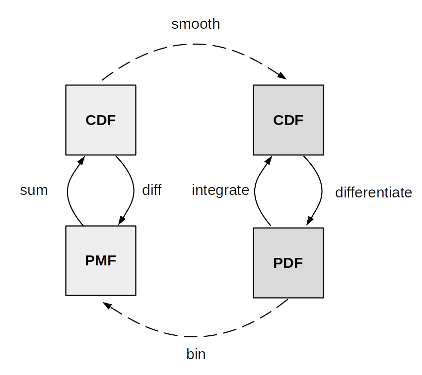
Fig. 175 summarize the relationship between the CDF, PDF and PMF. The transformations between discrete CDF and PMF on one side and continuous CDF and PMF on the other are well defined and thus we used arrows with solid lines. Instead the transformations between discrete and continuous variables are more about numerical approximation than well defined mathematical operations. To approximately get from a discrete to a continuous distribution we use a smoothing method. One form of smoothing is to use a continuous distribution instead of a discrete one. To go from continuous to discrete we can discretize or bin the continuous outcomes. For example, a Poisson distribution with a large value of \(\mu\) approximately Gaussian 10, while still being discrete. For those cases using a scenarios using a Poisson or a Gaussian maybe be interchangeable from a practical point of view. Using ArviZ you can use az.plot_kde with discrete data to approximate a continuous functions, how nice the results of this operation look depends on many factors. As we already said it may look good for a Poisson distribution with a relatively large value of \(\mu\). When calling az.plot_bpv(.) for a discrete variable, ArviZ will smooth it, using an interpolation method, because the probability integral transform only works for continuous variables.

Fig. 175 Relationship between the CDF, PDF and PMF. Adapted from the book Think Stats [131].¶

As we did with the discrete random variables, now we will see a few example of continuous random variables with their PDF and CDF.

( 1 ) 连续型均匀分布¶

A continuous random variable is said to have a Uniform distribution on the interval \((a, b)\) if its PDF is:

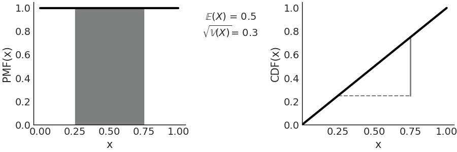
\[\begin{split}p(x \mid a,b)=\begin{cases} \frac{1}{b-a} & if a \le x \le b \\ 0 & \text{otherwise} \end{cases}\end{split}\]

Fig. 176 \(\mathcal{U}(0, 1)\) On the left the PDF, the black line represents the probability density, the gray shaded area represents the probability \(P(0.25 < X < 0.75) =0.5\). On the right the CDF, the height of the gray continuous segment represents \(P(0.25 < X < 0.75) =0.5\). Values outside of the support of the distribution are not represented.¶

The most commonly used Uniform distribution in statistics is \(\mathcal{U}(0, 1)\) also known as the standard Uniform. The PDF and CDF for the standard Uniform are very simple: \(p(x) = 1\) and \(F_{(x)} = x\) respectively, Fig. 176 represents both of them, this figure also indicated how to compute probabilities from the PDF and CDF.

( 2 ) 高斯（正态）分布¶

This is perhaps the best known distribution 11. On the one hand, because many phenomena can be described approximately using this distribution (thanks to central limit theorem, see Subsection ( 2 ) 中心极限定律 below). On the other hand, because it has certain mathematical properties that make it easier to work with it analytically.

The Gaussian distribution is defined by two parameters, the mean \(\mu\) and the standard deviation \(\sigma\) as shown in Equation (88). A Gaussian distribution with \(\mu=0\) and \(\sigma=1\) is known as the standard Gaussian distribution.

(88)¶\[ p (x \mid \mu, \sigma) = \frac {1} {\sigma \sqrt {2 \pi}} e^{-\frac {(x -\mu)^2} {2 \sigma^2}}\]

On the left panel of Fig. 177 we have the PDF, and on the right we have the CDF. Both the PDF and CDF are represented for the invertal -4, 4, but notice that the support of the Gaussian distribution is the entire real line.

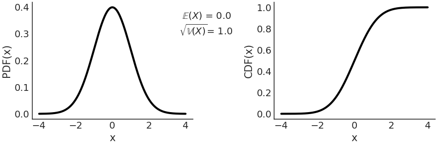
Fig. 177 Representation of \(\mathcal{N}(0, 1)\), on the left the PDF, on the right the CDF. The support of the Gaussian distribution is the entire real line.¶

( 3 ) 学生 \(t\) 分布¶

Historically this distribution arose to estimate the mean of a normally distributed population when the sample size is small 12. In Bayesian statistics, a common use case is to generate models that are robust against aberrant data as we discussed in Section 4.4 更稳健的回归.

\[p (x \mid \nu, \mu, \sigma) = \frac {\Gamma (\frac {\nu + 1} {2})} {\Gamma (\frac{\nu} {2}) \sqrt {\pi \nu} \sigma} \left (1+ \frac{1}{\nu} \left (\frac {x- \mu} {\sigma} \right)^2 \right)^{-\frac{\nu + 1}{2}}\]

where \(\Gamma\) is the gamma function 13 and \(\nu\) is commonly called degrees of freedom. We also like the name degree of normality, since as \(\nu\) increases, the distribution approaches a Gaussian. In the extreme case of \(\lim_{\nu \to \infty}\) the distribution is exactly equal to a Gaussian distribution with the same mean and standard deviation equal to \(\sigma\).

When \(\nu=1\) we get the Cauchy distribution 14. Which is similar to a Gaussian but with tails decreasing very slowly, so slowly that this distribution does not have a defined mean or variance. That is, it is possible to calculate a mean from a data set, but if the data came from a Cauchy distribution, the spread around the mean will be high and this spread will not decrease as the sample size increases. The reason for this strange behavior is that distributions, like the Cauchy, are dominated by the tail behavior of the distribution, contrary to what happens with, for example, the Gaussian distribution.

For this distribution \(\sigma\) is not the standard deviation, which as already said could be undefined, \(\sigma\) is the scale. As \(\nu\) increases the scale converges to the standard deviation of a Gaussian distribution.

On the left panel of Fig. 178 we have the PDF, and on the right we have the CDF. Compare with Fig. 177, a standard normal and see how the tails are heavier for the Student T distribution with parameter \(\mathcal{T}(\nu=4, \mu=0, \sigma=1)\)

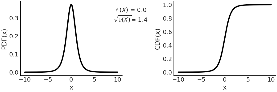
Fig. 178 \(\mathcal{T}(\nu=4, \mu=0, \sigma=1)\) On the left the PDF, on the right the CDF. The support of the Students T distribution is the entire real line.¶

( 4 ) 贝塔分布¶

The Beta distribution is defined in the interval \([0, 1]\). It can be used to model the behavior of random variables limited to a finite interval, for example, modeling proportions or percentages.

\[p (x \mid \alpha, \beta) = \frac {\Gamma (\alpha + \beta)} {\Gamma(\alpha) \Gamma (\beta)} \, x^{\alpha-1} (1 -x)^{\beta-1}\]

The first term is a normalization constant that ensures that the PDF integrates to 1. \(\Gamma\) is the Gamma function. When \(\alpha = 1\) and \(\beta = 1\) the Beta distribution reduces to the standard Uniform distribution. In Fig. 179 we show a \(\text{Beta}(\alpha=5, \beta=2)\) distribution.

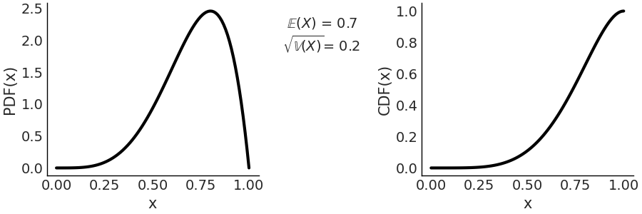
Fig. 179 \(\text{Beta}(\alpha=5, \beta=2)\) On the left the PDF, on the right the CDF. The support of the Beta distribution is on the interval \([0, 1]\).¶

If we want to express the Beta distribution as a function of the mean and the dispersion around the mean, we can do it in the following way.

\(\alpha = \mu \kappa\), \(\beta = (1 - \mu) \kappa\) where \(\mu\) the mean and \(\kappa\) a parameter called concentration as \(\kappa\) increases the dispersion decreases. Also note that \(\kappa = \alpha + \beta\).

11.1.6 联合分布、条件分布和边缘分布¶

假设我们有两个具有相同 PMF \(\text{Bin}(1, 0.5)\) 的随机变量 \(X\) 和 \(Y\)。他们是依赖的还是独立的？如果 \(X\) 代表抛硬币的正面，而 \(Y\) 代表另一次抛硬币的正面，那么它们是独立的。但是，如果它们在同一次抛硬币中分别代表正面和反面，那么它们是依赖的。因此，即使单个（正式称为单变量）PMF/PDF 完全表征单个随机变量，它们也没有关于单个随机变量如何与其他随机变量相关的信息。要回答这个问题，我们需要知道联合分布，也称为多元分布。如果我们认为 \(p(X)\) 提供了关于在实线上找到 \(X\) 的概率的所有信息，以类似的方式 \(p(X, Y)\)，\(X\) 和 \(Y 的联合分布\), 提供有关在平面上找到元组 \((X, Y)\) 的概率的所有信息。联合分布允许我们描述来自同一个实验的多个随机变量的行为，例如，后验分布是我们根据观测数据调整模型后模型中所有参数的联合分布。

The joint PMF is given by

\[p_{X,Y}(x, y) = P(X = x, Y = y)\]

\(n\) 离散随机变量的定义类似，我们只需要包含 \(n\) 项。与单变量 PMF 类似，有效的联合 PMF 必须是非负的并且总和为 1，其中总和取自所有可能的值。

\[\sum_x \sum_y P(X=x, Y=y) = 1\]

以类似的方式，\(X\) 和 \(Y\) 的联合 CDF 是

(89)¶\[F_{X,Y}(x, y) = P(X \le x, Y \le y)\]

给定 \(X\) 和 \(Y\) 的联合分布，我们可以通过对 \(Y\) 的所有可能值求和来得到 \(X\) 的分布：

\[P(X=x) = \sum_y P(X=x, Y=y)\]

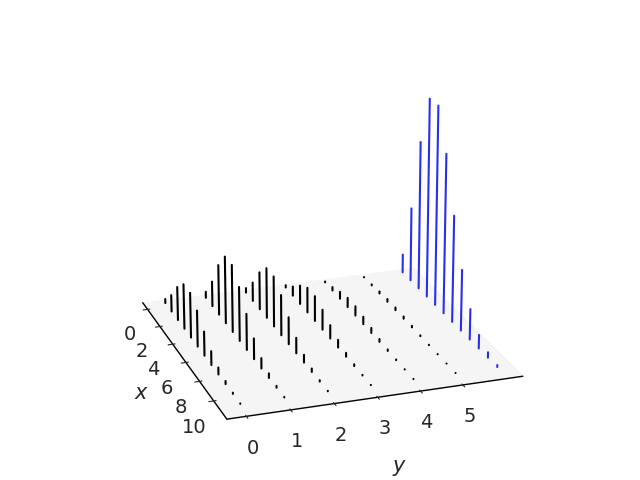
Fig. 180 黑线代表\(x\)和\(y\)的联合分布。 \(x\) 的边际分布中的蓝线是通过将 \(x\) 的每个值沿 y 轴的线的高度相加得到的。¶

在上一节中，我们将 \(P(X=x)\) 称为 \(X\) 的 PMF，或者只是 \(X\) 的分布，在处理联合分布时，我们通常将其称为 \(X\) 的边际分布。我们这样做是为了强调我们谈论的是个人 \(X\)，没有提及 \(Y\)。通过对 \(Y\) 的所有可能值求和，我们摆脱了 \(Y\)。

正式地，这个过程被称为边缘化 \(Y\) 。为了获得 \(Y\) 的 PMF，我们可以以类似的方式进行，但将 \(X\) 的所有可能值相加。在超过 2 个变量的联合分布的情况下，我们只需要对所有其他变量求和。 Fig. 180 说明了这一点。

鉴于联合分布，很容易获得边际。

但是，除非我们做出进一步的假设，否则从边缘到联合分布通常是不可能的。在 Fig. 180 中，我们可以看到只有一种方法可以沿 y 轴或 x 轴添加条形高度，但要反过来我们必须 split 个条形，并且有无限种方法使这种分裂。

我们已经在 11.1.2 条件概率节中介绍了条件分布，并且在 Fig. 169 中我们展示了条件化正在重新定义样本空间。

Fig. 181 演示了在 \(X\) 和 \(Y\) 联合分布的上下文中的条件反射。为了以 \(Y=y\) 为条件，我们采用 \(Y=y\) 值处的联合分布，而忽略其余部分。即那些 \(Y \ne y\)，这类似于索引二维数组并选择单个列或行。 \(X\) 的 remaining 值，Fig. 181 中的粗体值需要总和为 1 才能成为有效的 PMF，因此我们通过除以 \(P(Y=y)\) 重新归一化。

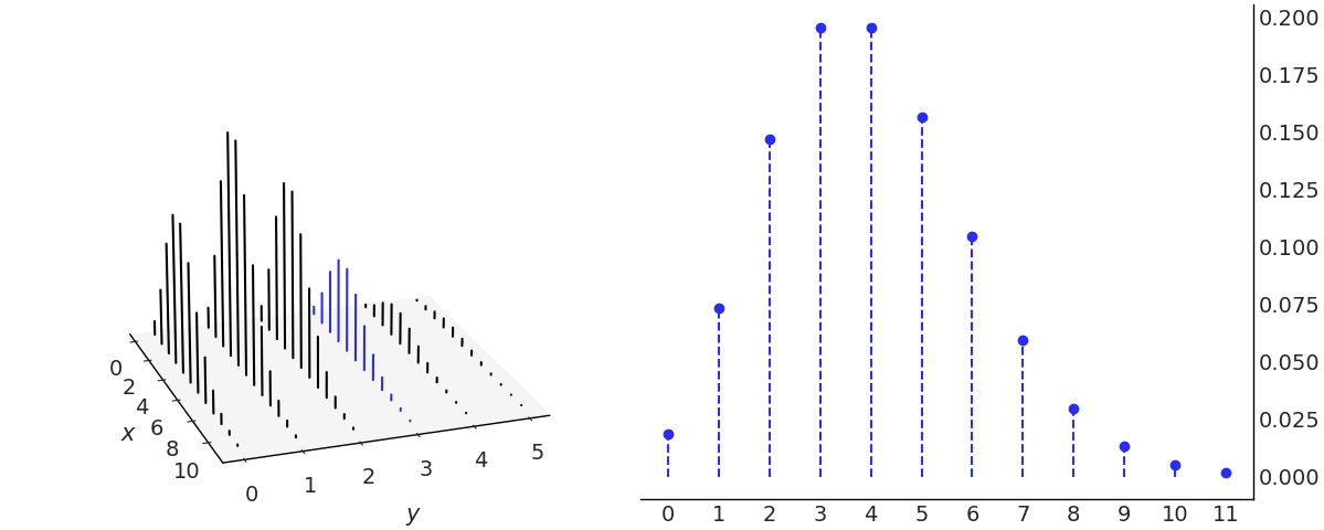
Fig. 181 左边是 \(x\) 和 \(y\) 的联合分布。蓝线代表条件分布 \(p(x \ mid y=3)\)。在右侧，我们分别绘制了相同的条件分布。请注意，\(x\) 的条件 PMF 与 \(y\) 的值一样多，反之亦然。我们只是强调一种可能性。¶

我们将连续联合 CDF 定义为方程 (89)，与离散变量相同，联合 PDF 作为 CDF 关于 \(x\) 和 \(y\) 的导数。我们要求有效的联合 PDF 是非负的并且积分为 1。对于连续变量，我们可以以与离散变量类似的方式将变量边缘化，不同之处在于我们需要计算积分而不是总和。

\[pdf_X(x) = \int pdf_{X,Y} (x, y)dy\]

../_images/joint_marginal_cond_continuous.png

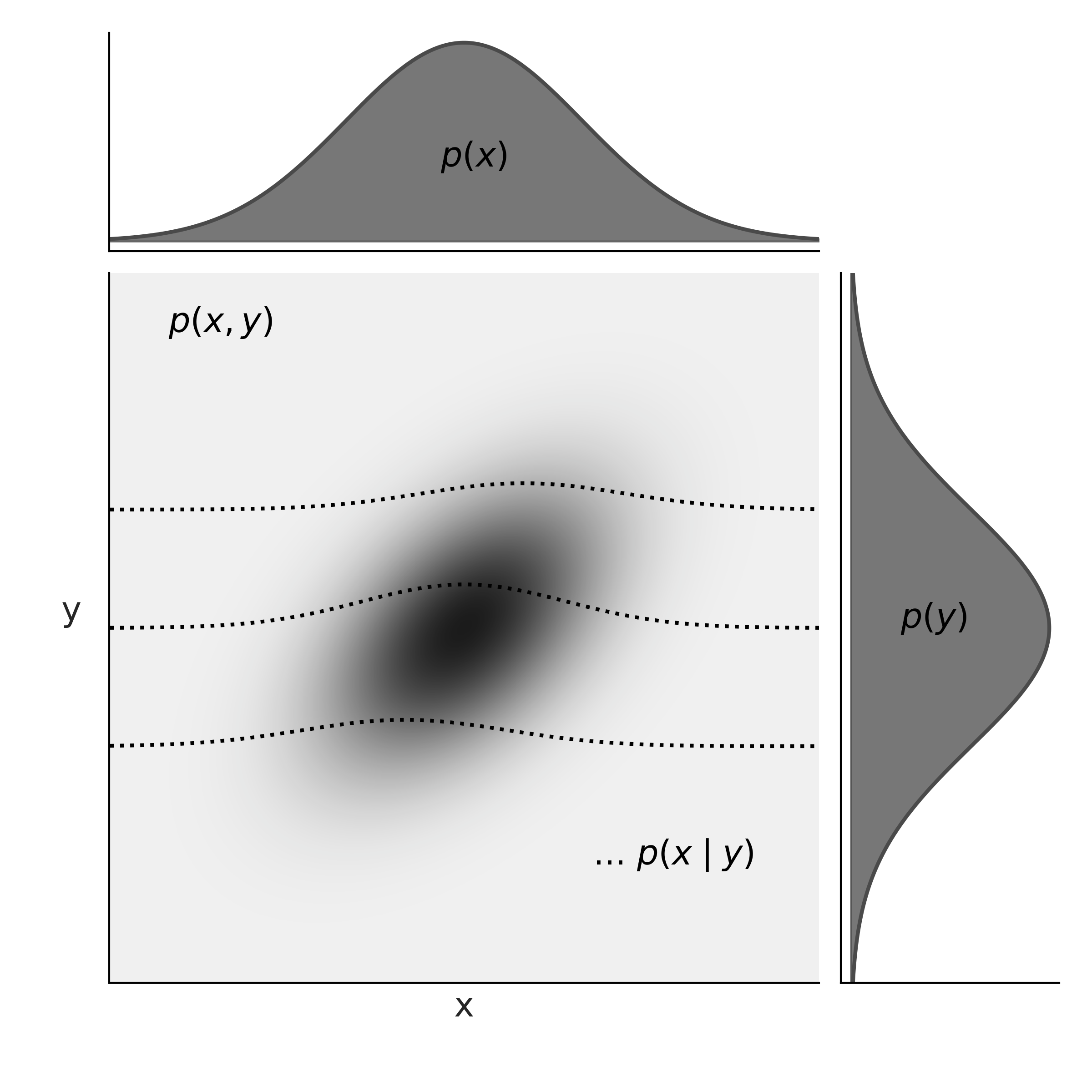
Fig. 182 在图的中心，我们有联合概率 \(p(x, y)\) 用灰度表示，概率密度越高越暗。在顶部和右侧 margins 我们分别有边际分布 \(p(x)\) 和 \(p(y)\)。虚线表示 3 个不同的 \(y\) 值的条件概率 \(p(x \mid y)\)。我们可以将这些视为在给定值 \(y\) 处的联合 \(p(x, y)\) 的（重新归一化的）切片。¶

Fig. 183 显示了另一个带有边缘分布的连接分布示例。这也是一个明显的例子，从联合到边缘很简单，因为有一种独特的方式来做这件事，但是除非我们引入进一步的假设，否则逆向是不可能的。联合分布也可以是离散分布和连续分布的混合。

Fig. 184 显示了一个示例。

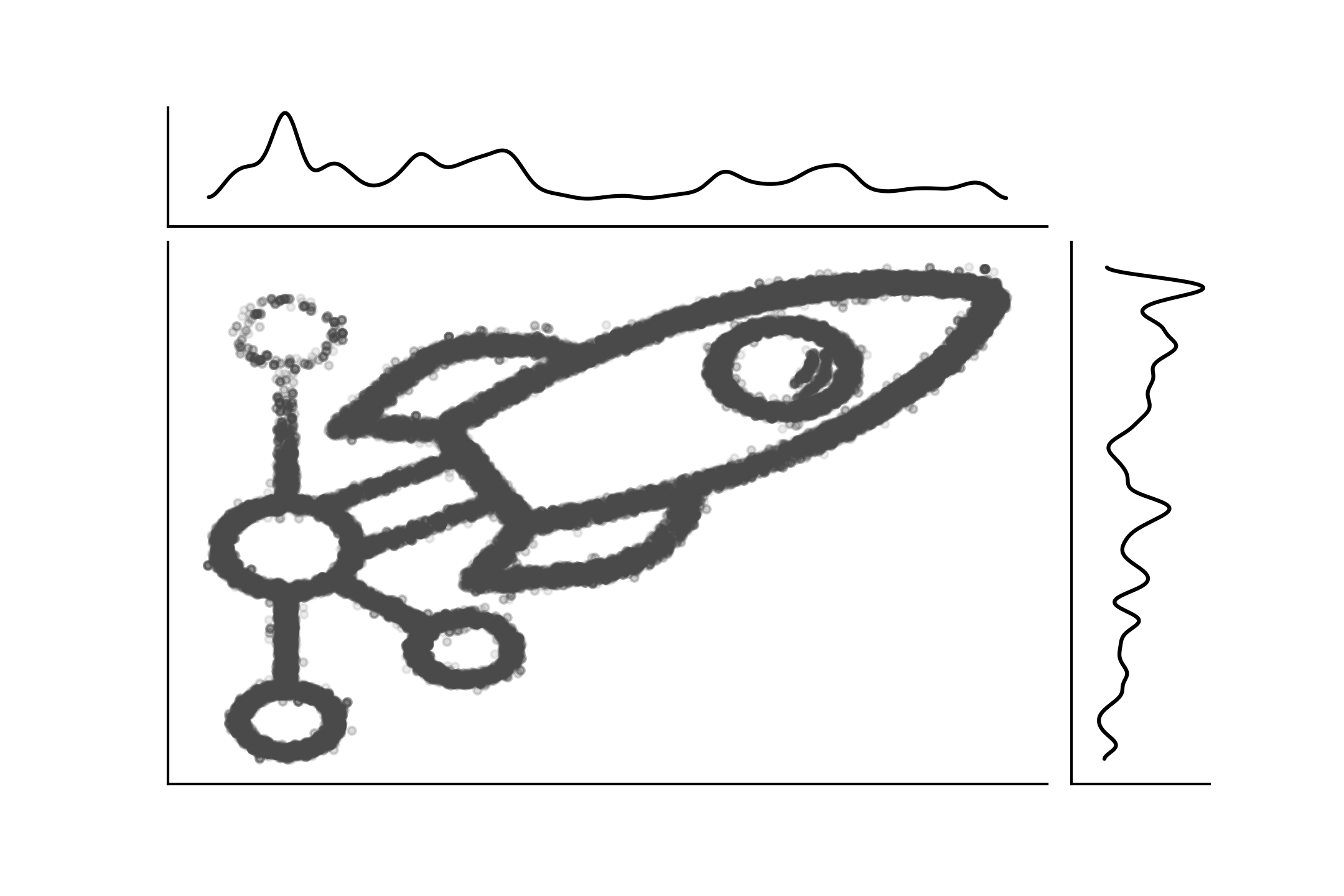
Fig. 183 PyMC3 徽标作为带有边缘的联合分布的样本。该图是使用 imcmc https://github.com/ColCarroll/imcmc 创建的，该库用于将 2D 图像转换为概率分布，然后从中采样以创建图像和 gif。¶

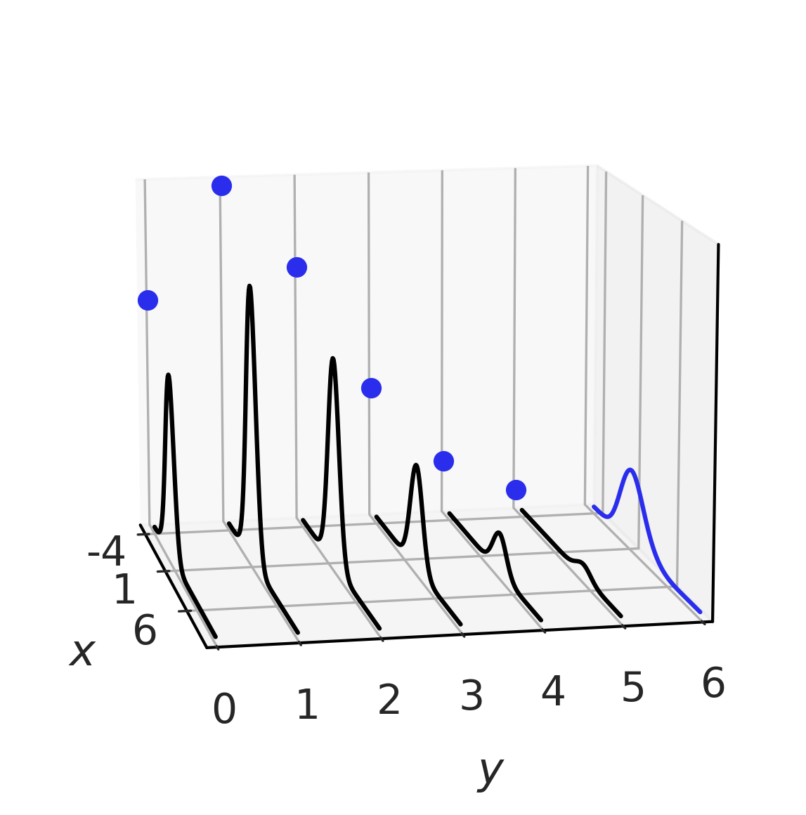
Fig. 184 黑色的混合联合分布。边际以蓝色表示，\(X\) 分布为高斯分布，\(Y\) 分布为泊松分布。很容易看出对于 \(Y\) 的每个值，我们如何具有（高斯）条件分布。¶

11.1.7 概率积分变换 (PIT)¶

概率积分变换 (PIT)，也称为均匀分布的普遍性，它指出给定具有连续分布的随机变量 \(X\)，具有累积分布 \(F_X\)，我们可以计算具有标准均匀分布的随机变量 \(Y\)分布为：

(90)¶\[Y = F_X (X)\]

通过 \(Y\) 的 CDF 的定义，我们可以看到这是真的

\[F_Y (y) = P(Y \leq y)\]

替换前一个中的方程 (90)

\[\begin{split}P(F_X (X) \leq y) \\\end{split}\]

取 \(F_X\) 的倒数到不等式的两边

\[\begin{split}P(X \leq F^{-1}_X (y)) \\\end{split}\]

根据 CDF 的定义

\[F_X (F^{-1}_X (y))\]

简化后，我们得到标准均匀分布 \(\mathcal{U}(0, 1)\) 的 CDF。

\[F_Y(y) = y\]

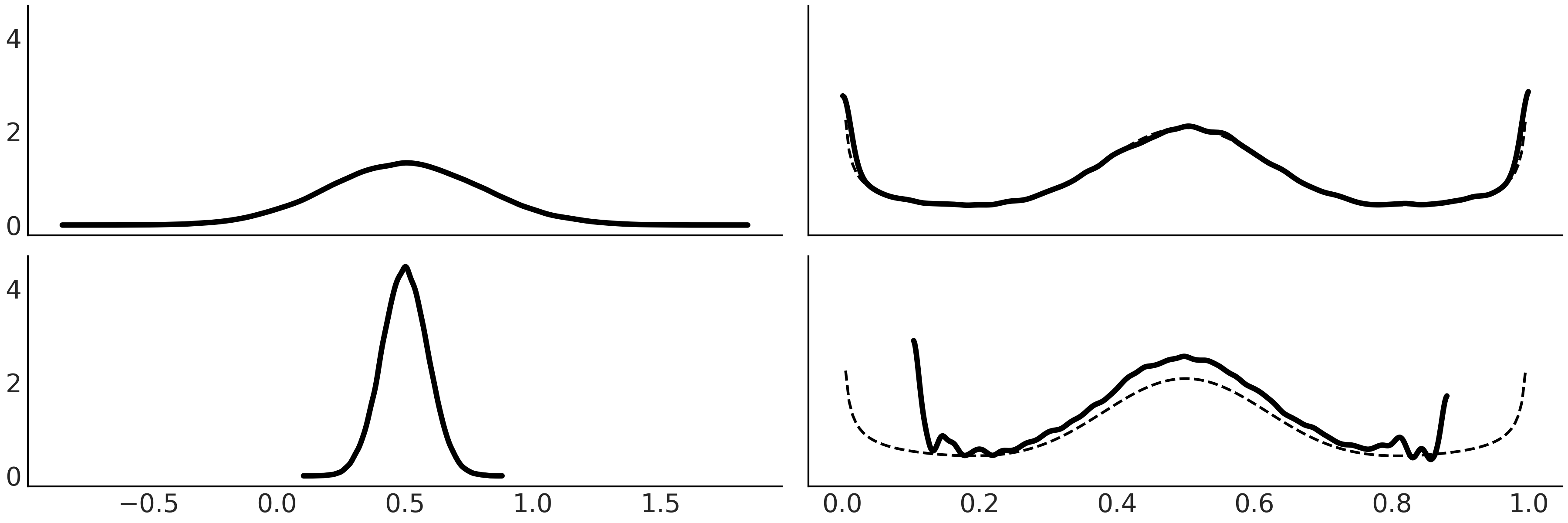
如果我们不知道 CDF \(F_X\) 但我们有来自 \(X\) 的样本，我们可以用经验 CDF 来近似它。 Fig. 185 显示了使用代码块 pit 生成的此属性的示例。

Listing 164 pit¶

xs = (np.linspace(0, 20, 200), np.linspace(0, 1, 200), np.linspace(-4, 4, 200))
dists = (stats.expon(scale=5), stats.beta(0.5, 0.5), stats.norm(0, 1))


_, ax = plt.subplots(3, 3)

for idx, (dist, x) in enumerate(zip(dists, xs)):
    draws = dist.rvs(100000)
    data = dist.cdf(draws)
    # PDF original distribution
    ax[idx, 0].plot(x, dist.pdf(x))
    # Empirical CDF
    ax[idx, 1].plot(np.sort(data), np.linspace(0, 1, len(data)))
    # Kernel Density Estimation
    az.plot_kde(data, ax=ax[idx, 2])

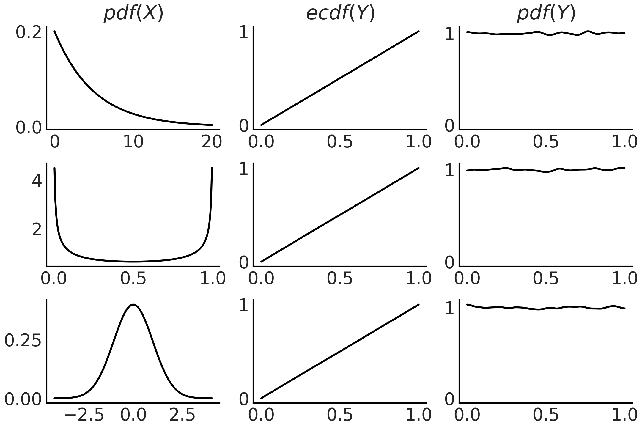
Fig. 185 在第一列，我们有 3 种不同分布的 PDF。为了生成中间列中的图，我们从相应的 PDF 中抽取 100000 次绘图，计算这些绘图的 CDF。我们可以看到这些是均匀分布的 CDF。最后一列与中间一列类似，不同之处在于我们使用核密度估计器来近似 PDF，而不是绘制经验 CDF，我们可以看到它近似于 Uniform。该图是使用代码块 pit 生成的。¶

概率积分变换用作测试的一部分，以评估给定数据集是否可以建模为来自指定分布（或概率模型）。在本书中，我们已经看到 PIT 在视觉测试 az.plot_loo_pit() 和 az.plot_pbv(kind="u_values") 后面使用。

PIT 也可用于从分布中采样。如果随机变量 \(X\) 分布为 \(\mathcal{U}(0,1)\)，则 \(Y = F^{-1}(X)\) 具有分布 \(F\)。因此，要从分布中获取样本，我们只需要（伪）随机数生成器，如“np.random.rand()”和感兴趣分布的逆 CDF。这可能不是最有效的方法，但它的通用性和简单性很难被击败。

11.1.8 期望¶

期望值是总结分布质心的单个数字。例如，如果 \(X\) 是一个离散随机变量，那么我们可以将其期望计算为：

\[\mathbb{E}(X) = \sum_x x P(X = x)\]

与统计中的常见情况一样，我们还希望测量分布的散布或离散度，例如，以表示像平均值这样的点估计周围的不确定性。我们可以用方差来做到这一点，这本身也是一种期望：

\[\mathbb{V}(X) = \mathbb{E}(X - \mathbb{E}X)^2 = \mathbb{E}(X^2 ) - (\mathbb{E}X)^2\]

在许多计算中，方差通常自然地出现，但要报告结果，取方差的平方根（称为标准差）通常更有用，因为它与随机变量的单位相同。

图 Fig. 172, Fig. 173, Fig. 174, Fig. 176, Fig. 177, fig:student_t_pdf_cdf 和 Fig. 179 显示了不同分布的期望值和标准差。

请注意，这些不是从样本计算的值，而是理论数学对象的属性。

期望是线性的，这意味着：

\[\mathbb{E}(cX) = c\mathbb{E}(X)\]

其中 \(c\) 是一个常数并且

\[\mathbb{E}(X + Y) = \mathbb{E}(X) + \mathbb{E}(Y)\]

即使在 \(X\) 和 \(Y\) 依赖的情况下也是如此。相反，方差不是线性的：

\[\mathbb{V}(cX) = c^2\mathbb{V}(X)\]

一般来说：

\[\mathbb{V}(X + Y) \neq \mathbb{V}(X) + \mathbb{V}(Y)\]

除非，例如，当 \(X\) 和 \(Y\) 是独立的。

我们将随机变量 \(X\) 的第 n 个矩表示为 \(\mathbb{E}(X^n)\)，因此期望值和方差也称为分布的一阶矩和二阶矩。第三个时刻，偏斜，告诉我们分布的不对称性。具有均值 \(\mu\) 和方差 \(\sigma^2\) 的随机变量 \(X\) 的偏度是 \(X\) 的第三个（标准化矩）：

\[\text{skew}(X) = \mathbb{E}\left(\frac{X -\mu}{\sigma}\right)^3\]

将偏斜计算为标准化量的原因，即减去均值并除以标准差是为了使偏斜独立于 \(X\) 的定位和规模，这是合理的，因为我们已经从均值中获得了该信息和方差，并且它会使偏度独立于 \(X\) 的单位，因此比较偏度变得更容易。

例如，\(\text{Beta}(2, 2)\) 的偏斜为 0，而 \(\text{Beta}(2, 5)\) 的偏斜为正，对于 \(\text{Beta}(5, 2 )\) 负数。对于单峰分布，正偏斜通常意味着右尾较长，而负偏斜则相反。

情况并非总是如此，原因是 0 偏斜意味着两侧尾部的总质量是平衡的。所以我们也可以通过一条又长又细的尾巴和另一条又短又肥的尾巴来平衡质量。

第四矩，称为峰度，告诉我们尾部的行为或极端值 [132]。它被定义为

(91)¶\[\text{Kurtosis}(X) = \mathbb{E}\left(\frac{X -\mu}{\sigma}\right)^4 - 3\]

减去 3 的原因是为了让高斯的峰度为 0，因为经常将峰度与高斯分布进行比较来讨论，但有时它通常在没有 \(-3\) 的情况下计算，所以当有疑问时问，或阅读，以了解在特定情况下使用的确切定义。通过检查方程 (91) 中的峰度定义，我们可以看到我们实际上是在计算标准化数据的四次方的期望值。因此，任何小于 1 的标准化值对峰度几乎没有任何贡献。相反，唯一有贡献的值是 extreme 值。

随着我们在 Student t 分布中增加 \(\nu\) 的值，峰度减小（高斯分布为零），并且随着我们减少 \(\nu\) 峰度增加。峰态仅在 \(\nu > 4\) 时定义，实际上对于 Student T 分布，第 \(n\) 时刻仅在 \(\nu > n\) 时定义。

SciPy 的 stats 模块提供了一种方法 stats(moments) 来计算分布的矩，正如你在代码块 scipy_unif 中看到的那样，它用于获取均值和方差。我们注意到，我们在本节中讨论的只是从概率分布而不是样本计算期望和矩，因此我们讨论的是理论分布的属性。当然，在实践中，我们通常希望从数据中估计分布的矩，因此统计学家有研究估计量，例如，样本均值和样本中位数是 \(\mathbb{E}(X)\) 的估计量。

11.1.9 变换¶

如果我们有一个随机变量 \(X\) 并且我们将函数 \(g\) 应用于它，我们将获得另一个随机变量 \(Y = g(X)\)。这样做之后，我们可能会问，既然我们知道 \(X\) 的分布，我们如何找出 \(Y\) 的分布。一种简单的方法是从 \(X\) 中采样并应用转换，然后绘制结果。但是当然有正式的方式来做到这一点。其中一种方法是应用变量更改技术。

如果 \(X\) 是一个连续随机变量并且 \(Y = g(X)\)，其中 \(g\) 是一个可微的严格递增或递减函数，则 \(Y\) 的 PDF 为：

(92)¶\[p_Y(y) = p_X(x) \left| \frac{dx}{dy} \right|\]

我们可以看到这是正确的，如下所示。令 \(g\) 严格递增，则 \(Y\) 的 CDF 为：

\[\begin{split}\begin{split} F_Y(y) =& P(Y \le y) \\ =& P(g(X) \le y) \\ =& P(X \le g^{-1}(y)) \\ =& F_X(g^{-1}(y)) \\ =& F_X(x) \\ \end{split}\end{split}\]

然后通过链式法则，\(Y\) 的 PDF 可以从 \(X\) 的 PDF 计算为：

\[p_Y(y) = p_X(x) \frac{dx}{dy}\]

\(g\) 严格递减的证明是相似的，但我们最终在右手项上有一个减号，因此我们在方程 (92) 中计算绝对值的原因。

对于多元随机变量（即更高维度）而不是导数，我们需要计算雅可比行列式，因此通常引用术语 \(\left| \frac{dx}{dy} \right|\) 即使在一维情况下也是雅可比行列式。点 \(p\) 的雅可比行列式的绝对值为我们提供了函数 \(g\) 在 \(p\) 附近扩大或缩小交易量的因子。雅可比行列式的这种解释也适用于概率密度。如果变换 \(g\) 不是线性的，那么受影响的概率分布将在某些区域缩小并在其他区域扩大。因此，当从已知的 PDF 中的 \(X\) 计算 \(Y\) 时，我们需要适当地考虑这些变形。像下面这样稍微重写方程 (92) 也有帮助：

\[p_Y(y)dy = p_X(x)dx\]

正如我们现在可以看到的，在微小的区间 \(p_Y(y)dy\) 中找到 \(Y\) 的概率等于在微小的区间 \(p_X(x)dx\) 中找到 \(X\) 的概率。所以雅可比行列式告诉我们如何将与 \(X\) 相关联的空间中的概率与与 \(Y\) 相关联的概率重新映射。

11.1.10 极限¶

两个最著名和最广泛使用的概率定理是大数定律和中心极限定理。它们都告诉我们随着样本量的增加，样本均值会发生什么变化。它们都可以在重复实验的背景下被理解，其中实验的结果可以被视为来自某些潜在分布的样本。

( 1 ) 大数定律¶

大数定律告诉我们，一个独立同分布随机变量的样本均值随着样本数量的增加而收敛到随机变量的期望值。对于某些分布，例如柯西分布（没有均值或有限方差），情况并非如此。

大数定律经常被误解，导致赌徒谬误。这种悖论的一个例子是相信在彩票中投注一个很长时间没有出现的号码是明智的。这里的错误推理是，如果某个特定数字有一段时间没有出现，那么一定有某种力量会增加该数字在下一次抽取中出现的概率。重新建立数字的等概率性和宇宙的自然秩序的力量。

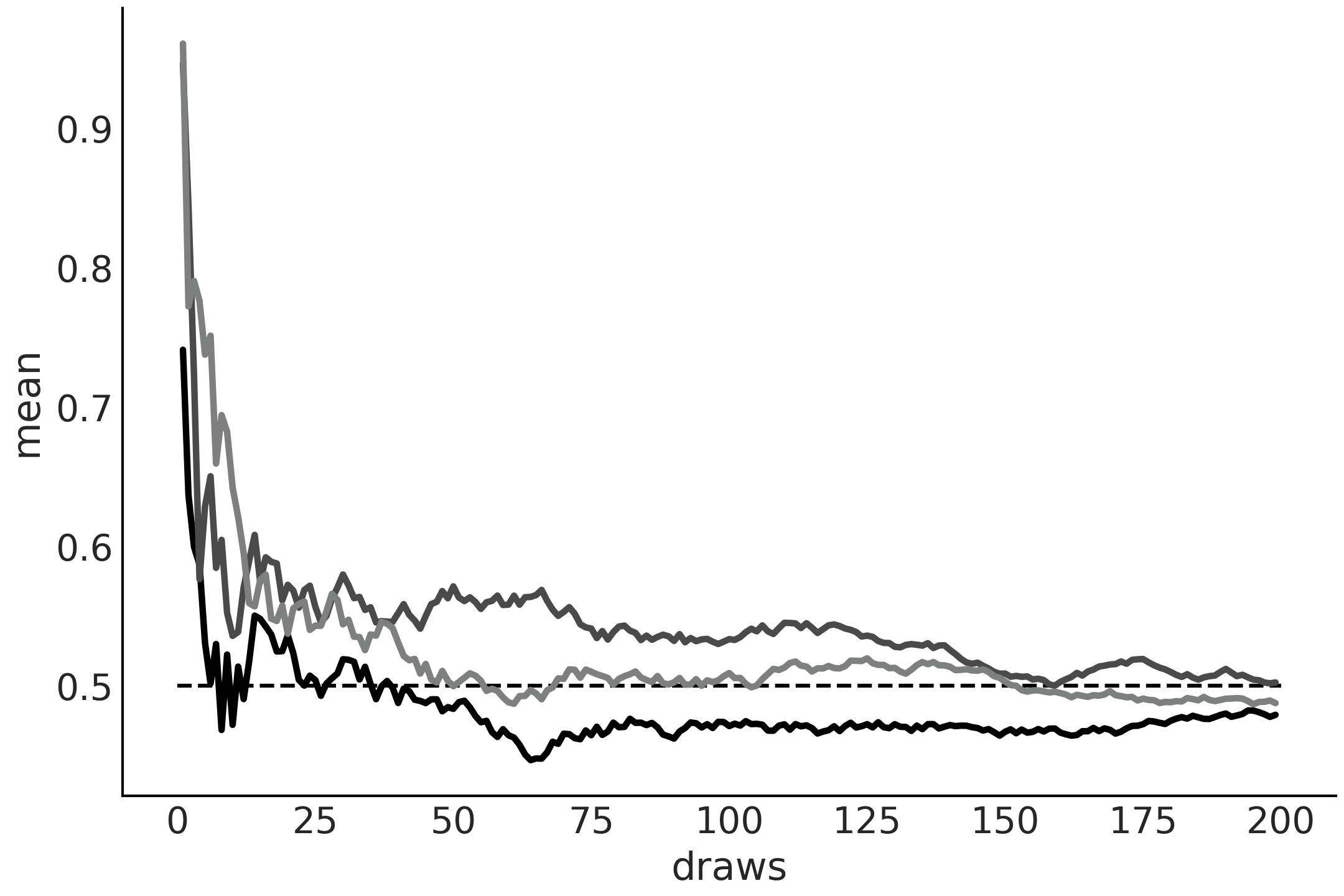
Fig. 186 来自 \(\mathcal{U}(0, 1)\) 分布的运行值。 0.5 处的虚线表示预期值。随着抽样次数的增加，经验均值接近预期值。每条线代表一个不同的样本。¶

( 2 ) 中心极限定律¶

中心极限定理指出：如果我们从任意分布中独立地采样得到 \(n\) 个值，则随着 \({n \rightarrow \infty}\) ，这些采样点的均值 \(\bar X\) 将近似呈高斯分布：

(93)¶\[\bar X_n \dot \sim \mathcal{N} \left (\mu, \frac{\sigma^2} {n} \right)\]

其中 \(\mu\) 和 \(\sigma^2\) 是任意分布的均值和方差。

为了满足中心极限定理，必须满足以下假设：

这些值是独立采样的
每个值都来自相同的分布
分布的均值和标准差必须是有限的

标准 1 和 2 可以放宽一些相当多，我们仍然会得到大致的高斯分布，但没有办法摆脱标准 3。对于没有定义均值或方差的分布，例如 Cauchy 分布，这个定理不适用。来自 Cauchy 分布的 \(N\) 值的均值不遵循高斯分布，而是遵循 Cauchy 分布。

中心极限定理解释了自然界中高斯分布的普遍性。我们研究的许多现象可以解释为围绕均值的波动，或者是许多不同因素总和的结果。

Fig. 187 显示了 3 种不同分布的中心极限定理，\(\text{Pois}(2.3)\), \(\mathcal{U}(0, 1)\), \(\text{Beta} (1, 10)\)，随着 \(n\) 的增加。

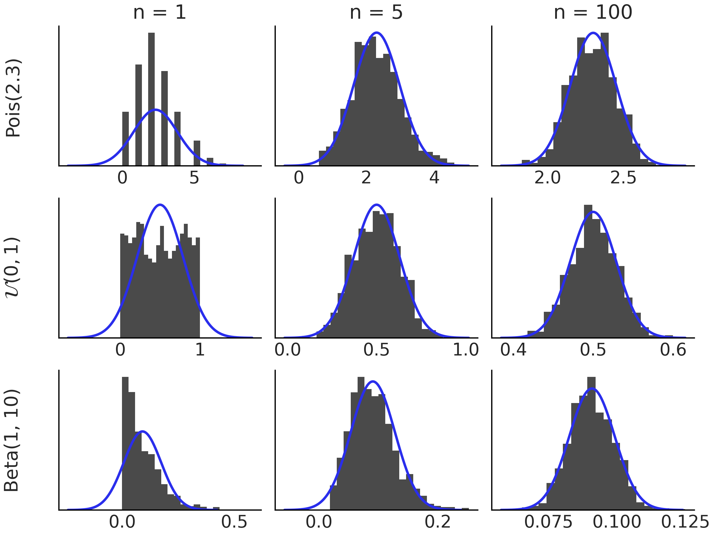
Fig. 187 左边距显示的分布直方图。每个直方图基于 \(\bar{X_n}\) 的 1000 个模拟值。随着我们增加 \(n\)，\(\bar{X_n}\) 的分布接近高斯分布。黑色曲线对应于根据中心极限定理的高斯分布。¶

11.1.11 马尔可夫链¶

A Markov Chain is a sequence of random variables \(X_0, X_1, \dots\) for which the future state is conditionally independent from all past ones given the current state. In other words, knowing the current state is enough to know the probabilities for all future states. This is known as the Markov property and we can write it as:

(94)¶\[P(X_{n+1} = j \mid X_n = i, X_{n-1} = i_{n-1} , \dots, X_0 = i_0) = P(X_{n+1} = j \mid X_n = i)\]

A rather effective way to visualize Markov Chains is imagining you or some object moving in space 15. The analogy is easier to grasp if the space is finite, for example, moving a piece in a square board like checkers or a salesperson visiting different cities. Given this scenarios you can ask questions like, how likely is to visit one state (specific squares in the board, cities, etc)? Or maybe more interesting if we keep moving from state to state how much time will we spend at each state in the long-run?

Fig. 188 shows four examples of Markov Chains, the first one show a classical example, an oversimplified weather model, where the states are rainy or sunny, the second example shows a deterministic die. The last two example are more abstract as we have not assigned any concrete representation to them.

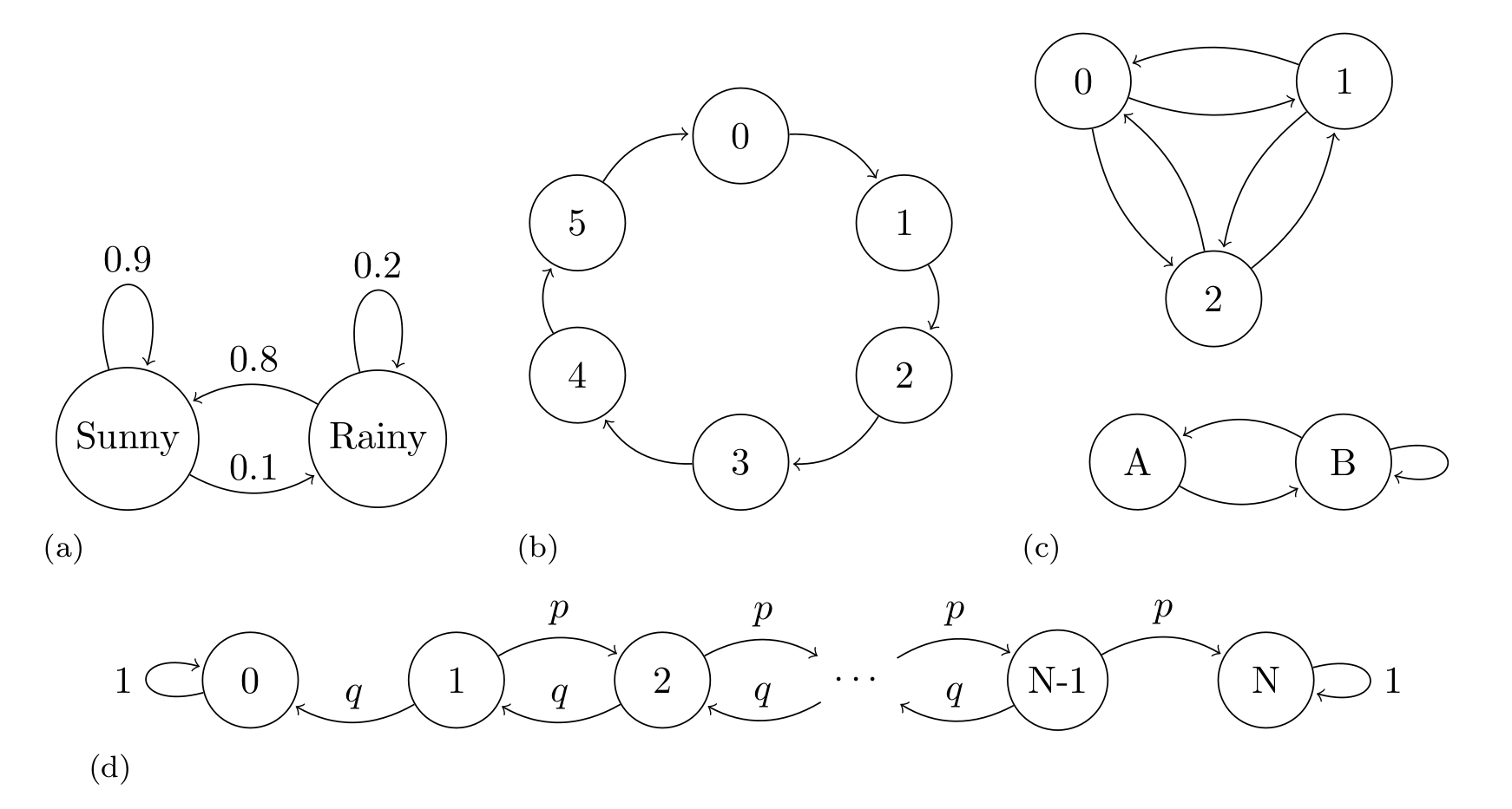
Fig. 188 Markov Chains examples. (a) An oversimplified weather model, representing the probability of a rainy or sunny day, the arrows indicate the transition between states, the arrows are annotated with their corresponding transition probabilities. (b) An example of periodic Markov Chain. (c) An example of a disjoint chain. The states 1, 2, and 3 are disjoint from states A and B. If we start at the state 1, 2, or 3 we will never reach state A or B and vice versa. Transition probabilities are omitted in this example. (d) A Markov chain representing the gambler’s ruin problem, two gamblers, A and B, start with \(i\) and \(N-i\) units of money respectively. At any given money they bet 1 unit, gambler A has probability \(p\) of and probability \(q = 1 - p\) of losing. If \(X_n\) is the total money of gambler A at time \(n\). Then \(X_0, X_1, \dots\) is a Markov chain as the one represented.¶

A convenient way to study Markov Chains is to collect the probabilities of moving between states in one step in a transition matrix \(\mathbf{T} = (t_{ij})\). For example, the transition matrix of example A in Fig. 188 is

\[\begin{split}\begin{bmatrix} 0.9 & 0.1 \\ 0.8 & 0.2 \end{bmatrix}\end{split}\]

and, for example, the transition matrix of example B in Fig. 188 is

\[\begin{split}\begin{bmatrix} 0 & 0 & 1 & 0 & 0 & 0 & 0 \\ 1 & 0 & 0 & 1 & 0 & 0 & 0 \\ 2 & 0 & 0 & 0 & 1 & 0 & 0 \\ 3 & 0 & 0 & 0 & 0 & 1 & 0 \\ 4 & 0 & 0 & 0 & 0 & 0 & 1 \\ 5 & 1 & 0 & 0 & 0 & 0 & 0 \\ \end{bmatrix}\end{split}\]

The \(i\)th row of the transition matrix represents the conditional probability distribution of moving from state \(X_{n}\) to the state \(X_{n+1}\). That is, \(p(X_{n+1} \mid X_n = i)\). For example, if we are at state sunny we can move to sunny (i.e. stay at the same state) with probability 0.9 and move to state rainy with probability 0.1. Notice how the total probability of moving from sunny to somewhere is 1, as expected for a PMF.

Because of the Markov property we can compute the probability of \(n\) consecutive steps by taking the \(n\)th power of \(\mathbf{T}\).

We can also specify the starting point of the Markov chain, i.e. the initial conditions \(s_i = P(X_0 = i)\) and let \(\mathbf{s}=(s_1, \dots, s_M)\). With this information we can compute the marginal PMF of \(X_n\) as \(\mathbf{s}\mathbf{T}^n\).

When studying Markov chains it makes sense to define properties of individual states and also properties on the entire chain. For example, if a chain returns to a state over and over again we call that state recurrent. Instead a transient state is one that the chain will eventually leave forever, in example (d) in Fig. 188 all states other than 0 or \(N\) are transient. Also, we can call a chain irreducible if it is possible to get from any state to any other state in a finite number of steps example (c) in Fig. 188 is not irreducible, as states 1,2 and 3 are disconnected from states A and B.

Understanding the long-term behavior of Markov chains is of interest. In fact, they were introduced by Andrey Markov with the purpose of demonstrating that the law of large numbers can be applied also to non-independent random variables. The previously mentioned concepts of recurrence and transience are important for understanding this long-term run behavior. If we have a chain with transient and recurrent states, the chain may spend time in the transient states, but it will eventually spend all the eternity in the recurrent states. A natural question we can ask is how much time the chain is going to be at each state. The answer is provided by finding the stationary distribution of the chain.

For a finite Markov chain, the stationary distribution \(\mathbf{s}\) is a PMF such that \(\mathbf{s}\mathbf{T} = \mathbf{s}\) 16. That is a distribution that is not changed by the transition matrix \(\mathbf{T}\).

Notice that this does not mean the chain is not moving anymore, it means that the chain moves in such a way that the time it will spend at each state is the one defined by \(\mathbf{s}\). Maybe a physical analogy could helps here. Imagine we have a glass not completely filled with water at a given temperature. If we seal it with a cover, the water molecules will evaporate into the air as moisture. Interestingly it is also the case that the water molecules in the air will move to the liquid water.

Initially more molecules might be going one way or another, but at a given point the system will find a dynamic equilibrium, with the same amount of water molecules moving to the air from the liquid water, as the number of water molecules moving from the liquid water to the air.

In physics/chemistry this is called a steady-state, locally things are moving, but globally nothing changes 17. Steady state is also an alternative name to stationary distribution.

Interestingly, under various conditions, the stationary distribution of a finite Markov chain exists and is unique, and the PMF of \(X_n\) converges to \(\mathbf{s}\) as \(n \to \infty\). Example (d) in Fig. 188 does not have a unique stationary distribution. We notice that once this chain reaches the states 0 or \(N\), meaning gambler A or B lost all the money, the chain stays in that state forever, so both \(s_0=(1, 0, \dots , 0)\) and \(s_N=(0, 0, \dots , 1)\) are both stationary distributions. On the contrary example B in Fig. 188 has a unique stationary distribution which is \(s=(1/6, 1/6, 1/6, 1/6, 1/6, 1/6)\), event thought the transition is deterministic.

If a PMF \(\mathbf{s}\) satisfies the reversibility condition (also known as detailed balance), that is \(s_i t_{ij} = s_j t_{ji}\) for all \(i\) and \(j\), we have the guarantee that \(\mathbf{s}\) is a stationary distribution of the Markov chain with transition matrix \(\mathbf{T} = t_{ij}\). Such Markov chains are called reversible. In Section 11.9 推断方法 we will use this property to show why Metropolis-Hastings is guaranteed to, asymptotically, work.

Markov chains satisfy a central limit theorem which is similar to Equation (93) except that instead of dividing by \(n\) we need to divide by the effective sample size (ESS). In Section 2.4.1 有效样本数量（ ESS ） we discussed how to estimate the effective sample size from a Markov Chain and how to use it to diagnose the quality of the chain. The square root of \(\frac{\sigma^2} {\text{ESS}}\) is the Monte Carlo standard error (MCSE) that we also discussed in Section 2.4.3 蒙特卡洛标准误差.

11.2 熵¶

In the Zentralfriedhof, Vienna, we can find the grave of Ludwig Boltzmann. His tombstone has the legend \(S = k \log W\), which is a beautiful way of saying that the second law of thermodynamics is a consequence of the laws of probability. With this equation Boltzmann contributed to the development of one of the pillars of modern physics, statistical mechanics. Statistical mechanics describes how macroscopic observations such as temperature are related to the microscopic world of molecules. Imagine a glass with water, what we perceive with our senses is basically the average behavior of a huge number water molecules inside that glass 18. At a given temperature there is a given number of arrangements of the water molecules compatible with that temperature (Figure Fig. 189). As we decrease the temperature we will find that less and less arrangements are possible until we find a single one. We have just reached 0 Kelvin, the lowest possible temperature in the universe! If we move into the other direction we will find that molecules can be found in more and more arrangements.

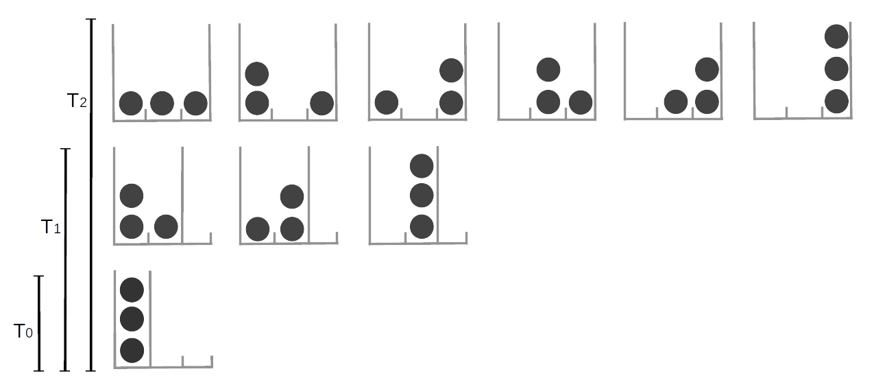
Fig. 189 The number of possible arrangements particles can take is related to the temperature of the system. Here we represent discrete system of 3 equivalent particles, the number of possible arrangements is represented by the available cells (gray high lines). increasing the temperature is equivalent to increasing the number of available cells. At \(T=0\) only one arrangement is possible, as the temperature increase the particles can occupy more and more states.¶

We can analyze this mental experiment in terms of uncertainty. If we know a system is at 0 Kelvin we know the system can only be in a single possible arrangement, our certainty is absolute 19, as we increase the temperature the number of possible arrangements will increase and then it will become more and more difficult to say, “Hey look! Water molecules are in this particular arrangement at this particular time!” Thus our uncertainty about the microscopic state will increase. We will still be able to characterize the system by averages such the temperature, volume, etc, but at the microscopic level the certainty about particular arrangements will decrease. Thus, we can think of entropy as a way of measuring uncertainty.

The concept of entropy is not only valid for molecules. It could also be applies to arrangements of pixels, characters in a text, musical notes, socks, bubbles in a sourdough bread and more. The reason that entropy is so flexible is because it quantifies the arrangements of objects - it is a property of the underlying distributions. The larger the entropy of a distribution the less informative that distribution will be and the more evenly it will assign probabilities to its events. Getting an answer of “\(42\)” is more certain than “\(42 \pm 5\)”, which again more certain than “any real number”. Entropy can translate this qualitative observation into numbers.

The concept of entropy applies to continue and discrete distributions, but it is easier to think about it using discrete states and we will see some example in the rest of this section. But keep in mind the same concepts apply to the continuous cases.

For a probability distribution \(p\) with \(n\) possible different events which each possible event \(i\) having probability \(p_i\), the entropy is defined as:

(95)¶\[H(p) = - \mathbb{E}[\log{p}] = -\sum_{i}^n p_i \log{p_i}\]

Equation (95) is just a different way of writing the entropy engraved on Boltzmann’s tombstone. We annotate entropy using \(H\) instead of \(S\) and set \(k=1\). Notice that the multiplicity \(W\) from Boltzmann’s version is the total number of ways in which different outcomes can possibly occur:

\[W = \frac{N!}{n_1!n_2! \cdots n_t!}\]

You can think of this as rolling a t-sided die \(N\) times, where \(n_i\) is the number of times we obtain side \(i\). As \(N\) is large we can use Stirling’s approximation \(x! \approx (\frac{x}{e})^x\).

\[W = \frac{N^N}{n_1^{n_1} n_2^{n_2} \cdots n_t^{n_t}} e^{(n_1 n_2 \cdots n_t-N)}\]

noticing that \(p_i = \frac{n_i}{N}\) we can write:

\[W = \frac{1}{p_1^{n_1} p_2^{n_2} \cdots p_t^{n_t}}\]

And finally by taking the logarithm we obtain

\[\log W = -\sum_{i}^n p_i \log{p_i}\]

which is exactly the definition of entropy.

We will now show how to compute entropy in Python using Code Block entropy_dist, with the result shown in Fig. 190.

Listing 165 entropy_dist¶

x = range(0, 26)
q_pmf = stats.binom(10, 0.75).pmf(x)
qu_pmf = stats.randint(0, np.max(np.nonzero(q_pmf))+1).pmf(x)
r_pmf = (q_pmf + np.roll(q_pmf, 12)) / 2
ru_pmf = stats.randint(0, np.max(np.nonzero(r_pmf))+1).pmf(x)
s_pmf = (q_pmf + np.roll(q_pmf, 15)) / 2
su_pmf = (qu_pmf + np.roll(qu_pmf, 15)) / 2

_, ax = plt.subplots(3, 2, figsize=(12, 5), sharex=True, sharey=True,
                     constrained_layout=True)
ax = np.ravel(ax)

zipped = zip([q_pmf, qu_pmf, r_pmf, ru_pmf, s_pmf, su_pmf],
             ["q", "qu", "r", "ru", "s", "su"])
for idx, (dist, label) in enumerate(zipped):
    ax[idx].vlines(x, 0, dist, label=f"H = {stats.entropy(dist):.2f}")
    ax[idx].set_title(label)
    ax[idx].legend(loc=1, handlelength=0)

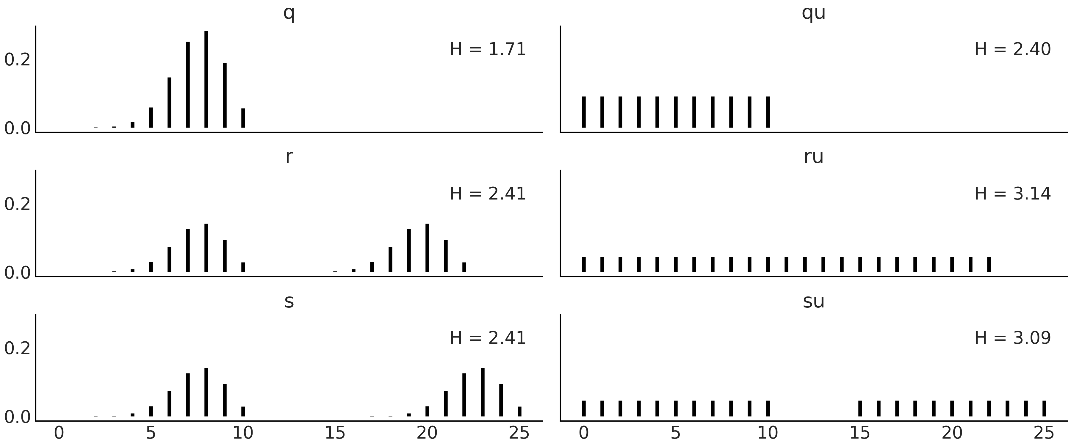
Fig. 190 Discrete distributions defined in Code Block entropy_dist and their entropy values \(H\).¶

Fig. 190 shows six distributions, one per subplot with its corresponding entropy. There are a lot of things moving on in this figure, so before diving in be sure to set aside an adequate amount of time (this maybe a good time to check your e-mails before going on). The most peaked, or least spread distribution is \(q\), and this is the distribution with the lowest value of entropy among the six plotted distributions. \(q \sim \text{binom}({n=10, p=0.75})\), and thus there are 11 possible events. \(qu\) is a Uniform distribution with also 11 possible events. We can see that the entropy of \(qu\) is larger than \(q\), in fact we can compute the entropy for binomial distributions with \(n=10\) and different values of \(p\) and we will see that none of them have larger entropy than \(qu\). We will need to increase \(n\) \(\approx 3\) times to find the first binomial distribution with larger entropy than \(qu\).

Let us move to the next row. We generate distribution \(r\) by taking \(q\) and shifting it to the right and then normalizing (to ensure the sum of all probabilities is 1). As \(r\) is more spread than \(q\) its entropy is larger. \(ru\) is the Uniform distribution with the same number of possible events as \(r\) (22), notice we are including as possible values those in the valley between both peaks. Once again the entropy of the Uniform version is the one with the largest entropy. So far entropy seems to be proportional to the variance of a distribution, but before jumping to conclusions let us check the last two distributions in Fig. 190. \(s\) is essentially the same as \(r\) but with a more extensive valley between both peaks and as we can see the entropy remains the same. The reason is basically that entropy does not care about those events in the valley with probability zero, it only cares about possible events. \(su\) is constructed by replacing the two peaks in \(s\) with \(qu\) (and normalizing). We can see that \(su\) has lower entropy than \(ru\) even when it looks more spread, after a more careful inspection we can see that \(su\) spread the total probability between fewer events (22) than \(ru\) (with 23 events), and thus it makes totally sense for it to have lower entropy.

11.3 KL 散度¶

统计学中常用一个概率分布\(q\)来表示另一个\(p\)，我们通常在不知道\(p\)但可以用\(q\)近似的情况下这样做。或者 \(p\) 很复杂，我们想找到一个更简单或更方便的分布 \(q\)。在这种情况下，我们可能会问通过使用 \(q\) 来表示 \(p\)，我们丢失了多少信息，或者等效地，我们引入了多少额外的不确定性。直观地说，我们希望数量只有在 \(q\) 等于 \(p\) 时才变为零，否则为正值。根据方程 (95) 中的熵定义，我们可以通过计算 \(\log(p)\) 和 \(\log(q)\) 之间的差值的期望值来实现这一点。这被称为 Kullback-Leibler (KL) 散度：

(96)¶\[\mathbb{KL}(p \parallel q) = \mathbb{E}_p[\log{p}-\log{q}]\]

因此，\(\mathbb{KL}(p \parallel q)\) 给出了当使用 \(q\) 来近似 \(p\) 时对数概率的平均差异。因为事件根据 \(p\) 出现在我们面前，我们需要计算关于 \(p\) 的期望。对于离散分布，我们有：

\[\mathbb{KL}(p \parallel q) = \sum_{i}^n p_i (\log{p_i} - \log{q_i})\]

使用对数属性，我们可以将其写成可能是表示 KL 散度的最常见方式：

\[\mathbb{KL}(p \parallel q) = \sum_{i}^n p_i \log{\frac{p_i}{q_i}}\]

我们还可以安排项并将 \(\mathbb{KL}(p \parallel q)\) 写为：

\[\mathbb{KL}(p \parallel q) = - \sum_{i}^n p_i (\log{q_i} - \log{p_i})\]

当我们扩展上述重新排列时，我们发现：

\[\mathbb{KL}(p \parallel q) = \overbrace{-\sum_{i}^n p_i \log{q_i}}^{H(p, q)} - \overbrace{\left(-\sum_{i}^n p_i \log{p_i}\right)}^{H(p)}\]

正如我们在上一节中已经看到的，\(H(p)\) 是 \(p\) 的熵。

\(H(p,q) = - \mathbb{E}_p[\log{q}]\) 类似于 \(q\) 的熵，但根据 \(p\) 的值进行评估。

重新排序上面我们得到：

\[H(p, q) = H(p) + D_\text{KL}(p \parallel q)\]

这表明，当使用 \(q\) 表示 \(p\) 时，KL 散度可以有效地解释为关于 \(H(p)\) 的额外熵。

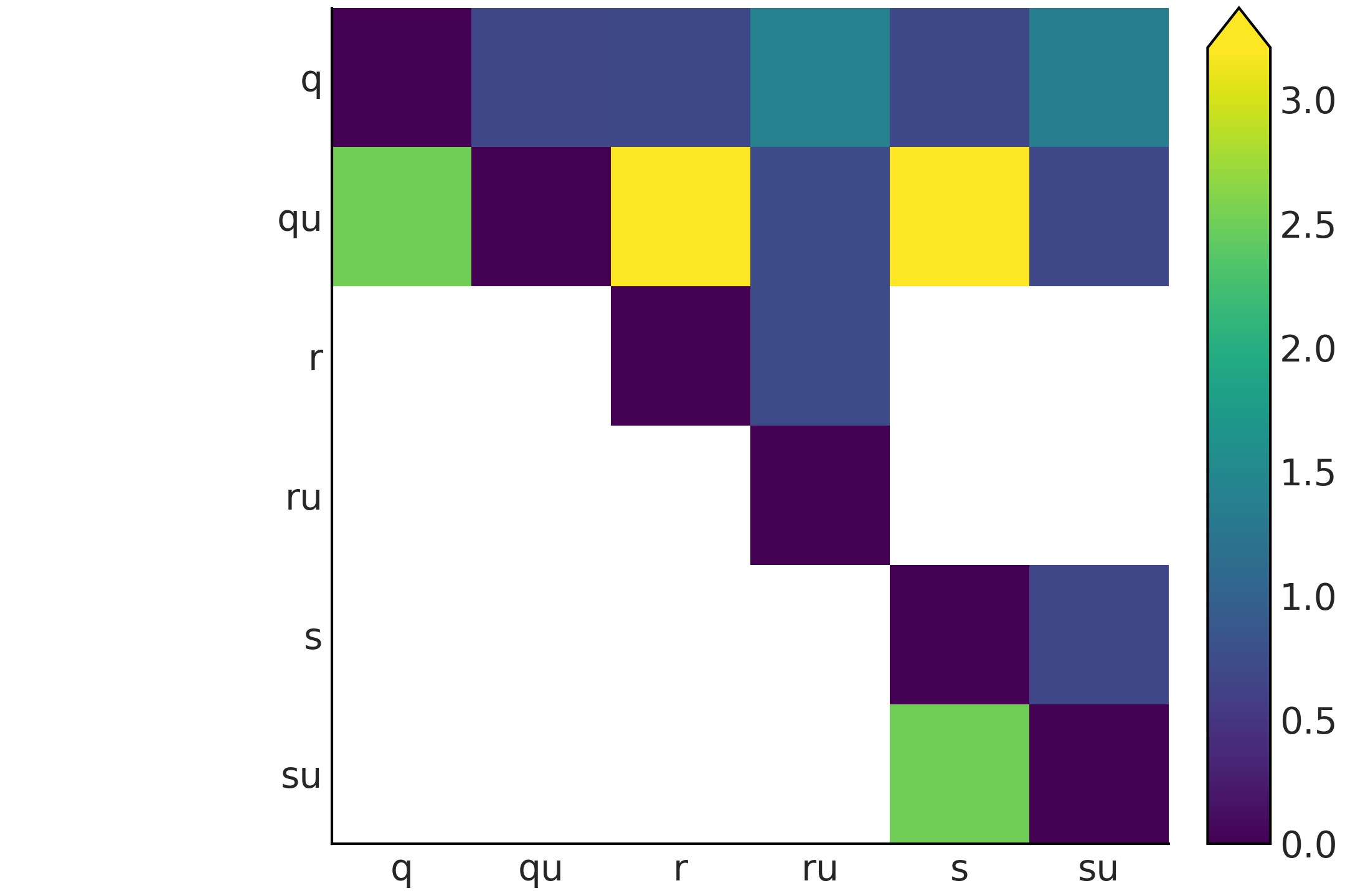
为了获得一点直觉，我们将计算 KL 散度的一些值并绘制它们。我们将使用与 Fig. 190 中相同的分布。

Listing 166 kl_varies_dist¶

dists = [q_pmf, qu_pmf, r_pmf, ru_pmf, s_pmf, su_pmf]
names = ["q", "qu", "r", "ru", "s", "su"]

fig, ax = plt.subplots()
KL_matrix = np.zeros((6, 6))
for i, dist_i in enumerate(dists):
    for j, dist_j in enumerate(dists):
        KL_matrix[i, j] = stats.entropy(dist_i, dist_j)

im = ax.imshow(KL_matrix, cmap="cet_gray")

代码块 kl_varies_dist 的结果显示在 Fig. 191 中。 Fig. 191 有两个特征立即弹出。首先，图形不是对称的，原因是\(\mathbb{KL}(p \parallel q)\)不一定和\(\mathbb{KL}(q \parallel p)\)一样。其次，我们有很多白细胞。它们代表 \(\infty\) 值。 KL 散度的定义使用以下约定 [133]：

\[0 \log \frac{0}{0} = 0, \quad 0 \log \frac{0}{q(\boldsymbol{x})} = 0, \quad p(\boldsymbol{x}) \log \frac{p(\boldsymbol{x})}{0} = \infty\]

Fig. 191 在 Fig. 190 中显示的分布 q、qu、r、ru、s 和 su 的所有成对组合的 KL 散度，白色用于表示无穷大值。¶

基于 KL 散度，我们可以激励使用对数分数来计算预期的对数逐点预测密度（在第 2 章方程 (20) 中介绍）。

让我们假设我们有 \(k\) 模型后验 \(\{q_{M_1}, q_{M_2}, \cdots q_{M_k}\}\)，让我们进一步假设我们知道 true 模型 \(M_0\) 然后我们可以计算：

\[\begin{split}\begin{split} \mathbb{KL}(p_{M_0} \parallel q_{M_1}) =&\; \mathbb{E}[\log{p_{M_0}}] - \mathbb{E}[\log{q_{M_1}}] \\ \mathbb{KL}(p_{M_0} \parallel q_{M_2}) =&\; \mathbb{E}[\log{p_{M_0}}] - \mathbb{E}[\log{q_{M_2}}] \\ &\cdots \\ \mathbb{KL}(p_{M_0} \parallel q_{M_k}) =&\; \mathbb{E}[\log{p_{M_0}}] - \mathbb{E}[\log{q_{M_k}}] \end{split}\end{split}\]

这似乎是一种徒劳的练习，因为在现实生活中我们不知道真正的模型 \(M_0\)。诀窍是要意识到 \(p_{M_0}\) 对于所有比较都是相同的，因此基于 KL-divergence 构建排名等同于基于 log-score 进行排名。

11.4 信息准则¶

信息标准是统计模型预测准确性的度量。它考虑了模型对数据的拟合程度并惩罚模型的复杂性。根据他们如何计算这两个术语，有许多不同的信息标准。最著名的家庭成员，尤其是对于非贝叶斯主义者，是 Akaike 信息准则 (AIC) [134]。它被定义为两项之和。 \(\log p(y_i \mid \hat{\theta}_{mle})\) 衡量模型对数据的拟合程度以及惩罚项 \(p_{AIC}\) 以说明我们使用相同数据的事实拟合模型并评估模型。

\[AIC = -2 \sum_{i}^{n} \log p(y_i \mid \hat{\theta}_{mle}) + 2 p_{AIC}\]

其中 \(\hat{\theta}_{mle}\) 是 \(\boldsymbol{\theta}\) 的最大似然估计，\(p_{AIC}\) 只是模型中参数的数量。

AIC 在非贝叶斯设置中非常流行，但不能很好地处理贝叶斯模型的一般性。它不使用完整的后验分布，因此丢弃了可能有用的信息。

平均而言，当我们从平面先验转向弱信息或信息先验时，和/或如果我们在模型中添加更多结构，比如分层模型，AIC 的表现会越来越差。 AIC 假设后验可以由高斯分布很好地表示（至少渐近地），但是对于许多模型来说，这并不正确，包括层次模型、混合模型、神经网络等。总之我们希望使用一些更好的备择方案。

广泛适用的信息准则 (WAIC 20) [135] 可以看作是 AIC 的完全贝叶斯扩展。它还包含两个术语，与 Akaike 标准的解释大致相同。最重要的区别是这些项是使用完整的后验分布计算的。

(97)¶\[WAIC = \sum_i^n \log \left(\frac{1}{s} \sum_{j}^S p(y_i \mid \boldsymbol{\theta}^j) \right) \; - \sum_i^n \left(\mathop{\mathbb{V}}_{j}^s \log p(Y_i \mid \boldsymbol{\theta}^j) \right)\]

方程 (97) 中的第一项只是 AIC 中的对数似然，但逐点评估，即在 \(n\) 观测值上的每个 \(i\) 观测数据点。我们通过取后验 \(s\) 样本的平均值来考虑后验的不确定性。第一项是计算公式 (19) 中定义的理论预期对数逐点预测密度 (ELPD) 及其在公式 (20) 中的近似值的实用方法。

第二项可能看起来有点奇怪，\(s\) 后验样本（每个观测）的方差也是如此。直观地，我们可以看到，对于每个观测，如果后验分布的对数似然相似，则方差会很低，如果后验分布中不同样本的对数似然变化更大，则方差会更大。我们发现对后验细节敏感的观测越多，惩罚就越大。我们也可以从另一个等效的角度来看待这一点；更灵活的模型是可以有效容纳更多数据集的模型。例如，包含直线但也包含向上曲线的模型比只允许直线的模型更灵活；因此，在后一个模型上评估的那些观测值的对数似然平均将具有更高的方差。如果更灵活的模型不能用更高的估计 ELPD 来补偿这种惩罚，那么我们会将更简单的模型列为更好的选择。因此，方程 (97) 中的方差项通过惩罚过于复杂的模型来防止过度拟合，并且可以松散地解释为 AIC 中的有效参数数量。

AIC 和 WAIC 都没有试图衡量模型是否真实，它们只是比较替代模型的相对衡量。

从贝叶斯的角度来看，先验是模型的一部分，但 WAIC 是在后验上评估的，并且先验效果只是通过影响结果后验的方式间接考虑在内。还有其他信息标准，如 BIC 和 WBIC，试图回答这个问题，可以看作是边际似然的近似值，但我们不会在本书中讨论它们。

11.5 深入理解留一交叉验证法¶

正如本书 2.5.2 交叉验证和留一法部分所讨论的，我们使用术语 LOO 来指代一种特定的方法来近似留一法交叉验证 (LOO-CV)，称为帕累托平滑重要性抽样留一法交叉验证(PSIS-LOO-CV)。在本节中，我们将讨论此方法的一些细节。

LOO 是 WAIC 的替代方案，实际上可以证明它们渐近收敛到相同的数值 [135, 136]。尽管如此，LOO 为从业者带来了两个重要的优势。它在有限样本设置中更加稳健，并且在计算期间提供有用的诊断 [16, 136]。

在 LOO-CV 下，新数据集的预期对数逐点预测密度为：

\[\text{ELPD}_\text{LOO-CV} = \sum_{i=1}^{n} \log \int \ p(y_i \mid \boldsymbol{\theta}) \; p(\boldsymbol{\theta} \mid y_{-i}) d\boldsymbol{\theta} \tag{\ref{eq:elpd_loo_cv}}\]

其中 \(y_{-i}\) 表示不包括 \(i\) 观测的数据集。

鉴于在实践中我们不知道 \(\boldsymbol{\theta}\) 的值，我们可以使用来自后验的 \(s\) 样本来近似方程 \(\ref{eq:elpd_loo_cv}\)：

(98)¶\[\sum_{i}^{n} \log \left(\frac{1}{s}\sum_j^s \ p(y_i \mid \boldsymbol{\theta_{-i}^j}) \right)\]

请注意，这个术语看起来类似于方程 (97) 中的第一项，除了我们每次都在计算 \(n\) 后验，删除一个观测值。因此，与 WAIC 相反，我们不需要添加惩罚项。在 (98) 中计算 \(\text{ELPD}_\text{LOO-CV}\) 非常昂贵，因为我们需要计算 \(n\) 后验。幸运的是，如果 \(n\) 观测是条件独立的，我们可以用方程 (99) [136, 137] 来近似方程 (98)：

(99)¶\[\text{ELPD}_{psis-loo} = \sum_i^n \log \sum_j^s w_i^j p(y_i \mid \boldsymbol{\theta}^j)\]

其中 \(w\) 是归一化权重的向量。

为了计算 \(w\)，我们使用了重要性抽样，这是一种估计感兴趣的特定分布 \(f\) 的属性的技术，因为我们只有来自不同分布 \(g\) 的样本。当从 \(g\) 采样比从 \(f\) 采样更容易时，使用重要性采样是有意义的。如果我们有一组来自随机变量 \(X\) 的样本，并且我们能够逐点评估 \(g\) 和 \(f\)，我们可以将重要性权重计算为：

(100)¶\[w_i = \frac{f(x_i)}{g(x_i)}\]

在计算上，它是这样的：

从 \(g\) 中抽取 \(N\) 个样本 \(x_i\)
计算每个样本的概率\(g(x_i)\)
在 \(N\) 个样本 \(f(x_i)\) 上评估 \(f\)
计算重要性权重 \(w_i = \frac{f(x_i)}{g(x_i)}\)
从 \(g\) 中返回 \(N\) 个样本，权重为 \(w\)、\((x_i, w_i)\)，可以插入到一些估计器中

Fig. 192 显示了使用两个不同的提案分布来近似相同目标分布（虚线）的示例。在第一行，提案比目标分布更宽。在第二行，提案比目标分布窄。正如我们所见，第一种情况下的近似值更好。这是重要性抽样的一般特征。

Fig. 192 重要性抽样。在左侧，我们有来自建议分布 \(g\) 的样本的 KDE，在右侧，虚线表示目标分布，实线表示在重新加权来自建议分布的样本后的近似分布，其权重计算如下(100)。¶

回到 LOO，我们计算的分布是后验分布。为了评估模型，我们需要从留一后验分布中抽取样本，因此我们要计算的重要性权重为：

\[w_i^j = \frac{p(\theta^j \mid y{-i} )}{p(\theta^j \mid y)} \propto \frac{1}{p(y_i \mid \theta^j)}\]

请注意，这种比例是个好消息，因为它允许我们几乎免费计算 \(w\)。但是，后验分布的尾部可能比留一法分布更细，正如我们在 Fig. 192 中看到的那样，这可能导致估计不佳。

从数学上讲，问题在于重要性权重可能具有很高甚至无限的方差。为了控制方差，LOO 应用了一个平滑过程，该过程涉及用估计的帕累托分布中的值替换最大的重要性权重。这有助于使 LOO 更加健壮 [136]。

此外，帕累托分布的估计 \(\hat\kappa\) 参数可用于检测高度影响的观测，即被排除在外时对预测分布有很大影响的观测值。通常，较高的 \(\hat \kappa\) 值可能表明数据或模型存在问题，尤其是当 \(\hat \kappa > 0.7\) [16, 22] 时。

11.6 Jeffreys 先验的推导¶

在本节中，我们将展示如何找到二项似然的 Jeffreys 先验，首先是成功次数参数 \(\theta\)，然后是几率参数 \(\kappa\)，其中 \(\kappa = \frac{\ theta}{1-\theta}\)。

回想一下第 1 章，对于 \(\theta\) 的一维情况 JP 定义为：

\[p(\theta) \propto \sqrt{I(\theta)}\]

其中 \(I(\theta)\) 是 Fisher 信息：

\[I(\theta) = - \mathbb{E_{Y}}\left[\frac{d^2}{d\theta^2} \log p(Y \mid \theta)\right]\]

11.6.1 依据 \(\theta\) 的二项似然 Jeffreys 先验¶

二项式似然可以表示为：

(101)¶\[p(Y \mid \theta) \propto \theta^{y} (1-\theta)^{n-y}\]

其中 \(y\) 是成功的次数，\(n\) 是试验的总数，因此 \(n-y\) 是失败的次数。我们写成比例，因为似然中的二项式系数不依赖于 \(\theta\)。

为了计算 Fisher 信息，我们需要取似然的对数：

\[\ell = \log(p(Y \mid \theta)) \propto y \log(\theta) + (n-y) \log(1-\theta)\]

然后计算二阶导数：

\[\begin{split}\begin{aligned} \begin{split} \frac{d \ell}{d\theta} &= \frac{y}{\theta} - \frac{n-y}{1-\theta} \\ \frac{d^{2} \ell}{d \theta^{2}} &= -\frac{y}{\theta^{2}} - \frac{n-y}{ (1-\theta)^{2}} \end{split}\end{aligned}\end{split}\]

Fisher 信息是似然二阶导数的期望值，则：

\[I(\theta) = - \mathbb{E}_{Y}\left[-\frac{y}{\theta^{2}} + \frac{n-y}{ (1-\theta)^{2}} \right]\]

由于 \(\mathbb{E}[y] = n\theta\)，我们可以写成：

\[I(\theta)= \frac{n\theta}{\theta^{2}} - \frac{n - n \theta}{(1-\theta)^{2}}\]

我们可以重写为：

\[I(\theta)= \frac{n}{\theta} - \frac{n (1 -\theta)}{(1-\theta)^{2}} = \frac{n}{\theta} - \frac{n}{(1-\theta)}\]

我们可以用一个共同的分母来表达这些分数，

\[I(\theta)= n \left[ \frac{1 - \theta}{\theta (1 - \theta)} - \frac{\theta}{\theta (1-\theta)}\right]\]

通过重组：

\[I(\theta) = n \frac{1}{\theta (1-\theta)}\]

如果我们省略 \(n\) 那么我们可以这样写：

(102)¶\[I(\theta) \propto \frac{1}{\theta (1-\theta)} = \theta^{-1} (1-\theta)^{-1}\]

最后，我们需要对方程 (102) 中的 Fisher 信息取平方根，从而得出二项式似然的 \(\theta\) 的 Jeffreys 先验如下：

(103)¶\[\begin{aligned} p(\theta) \propto \theta^{-0.5} (1-\theta)^{-0.5} \end{aligned}\]

11.6.2 依据 \(\kappa\) 的二项似然 Jeffreys 先验¶

现在让我们看看如何根据赔率 \(\kappa\) 获得二项式似然的 Jeffreys 先验。我们首先替换表达式 (101) 中的 \(\theta = \frac{\kappa}{\kappa + 1}\)：

\[p(Y \mid \kappa) \propto \left({\frac{\kappa}{\kappa + 1}}\right)^{y} \left(1-{\frac{\kappa}{\kappa +1}}\right)^{n-y}\]

也可以写成：

\[p(Y \mid \kappa) \propto \kappa^y (\kappa + 1)^{-y} (\kappa +1)^{-n + y}\]

并进一步简化为：

(104)¶\[p(Y \mid \kappa) \propto \kappa^y (\kappa + 1)^{-n}\]

现在我们需要取对数：

\[\ell = \log(p(Y \mid \kappa)) \propto y \log{\kappa} -n \log{(\kappa + 1)}\]

然后我们计算二阶导数：

\[\begin{split}\begin{aligned} \begin{split} \frac{d \ell}{d{\kappa}} &= \frac{y}{\kappa} - \frac{n}{\kappa + 1} \\ \frac{d^2 \ell}{d {\kappa^2}} &= -\frac{y}{\kappa^2} + \frac{n}{(\kappa+1)^2} \end{split}\end{aligned}\end{split}\]

Fisher 信息是似然二阶导数的期望值，则：

\[I(\kappa) = - \mathbb{E}_Y\left[-\frac{y}{\kappa^2} + \frac{n}{ (\kappa+1)^2} \right]\]

由于 \(\mathbb{E}[y] = n \theta = n \frac{\kappa}{\kappa + 1}\)，我们可以写成：

\[I(\kappa) = \frac{n}{\kappa (\kappa + 1)} - \frac{n}{(\kappa + 1)^2}\]

我们可以用一个共同的分母来表达这些分数，

\[I(\kappa) = \frac{n (\kappa + 1)}{\kappa (\kappa + 1)^2} - \frac{n \kappa}{\kappa (\kappa + 1)^2}\]

然后我们合并成一个分数：

\[I(\kappa) = \frac{n (\kappa + 1) - n \kappa}{\kappa (\kappa + 1)^2}\]

然后我们将 \(n\) 分配给 \((\kappa + 1)\) 并简化：

\[I(\kappa) = \frac{n}{\kappa (\kappa + 1)^2}\]

最后，通过取平方根，我们得到 Jeffreys 在由几率参数化时的二项似然先验：

(105)¶\[p(\kappa) \propto \kappa^{-0.5} (1 + \kappa)^{-1}\]

11.6.3 二项似然的 Jeffreys 后验¶

为了在根据 \(\theta\) 参数化似然性时获得 Jeffrey 的后验，我们可以将方程 (101) 与方程 (103) 结合起来

(106)¶\[p(\theta \mid Y) \propto \theta^{y} (1-\theta)^{n-y} \theta^{-0.5} (1-\theta)^{-0.5} = \theta^{y-0.5} (1-\theta)^{n-y-0.5}\]

类似地，当似然用 \(\kappa\) 参数化时，Jeffreys 的后验我们可以将 (104) 与 (105) 结合起来

(107)¶\[p(\kappa \mid Y) \propto \kappa^y (\kappa + 1)^{-n} \kappa^{-0.5} (1 + \kappa)^{-1} = \kappa^{(y-0.5)} (\kappa + 1)^{(-n-1)})\]

11.7 `边缘似然`¶

对于某些模型，例如使用共轭先验的模型，边缘似然在分析上是易于处理的。其余的，数值计算这个积分是出了名的困难，因为这涉及对通常复杂且高度可变的函数 [138] 的高维积分。在本节中，我们将尝试直观地了解为什么这通常是一项艰巨的任务。

在数值上，在低维度上，我们可以通过在网格上评估先验和似然的乘积，然后应用梯形规则或其他类似方法来计算边缘似然。正如我们将在 11.8 走出平地部分中看到的，使用网格不能很好地随维度缩放，因为随着模型中变量数量的增加，所需的网格点的数量会迅速增加。

因此，基于网格的方法对于具有多个变量的问题变得不切实际。蒙特卡洛积分也可能存在问题，至少在最简单的实现中是这样（参见第 11.8 走出平地节）。

出于这个原因，已经提出了许多专门的方法来计算边缘似然 [138]。这里我们只讨论其中之一。我们主要关心的不是学习如何在实践中计算边缘似然，而是说明为什么很难做到。

11.7.1 调和平均估计器¶

一个相当臭名昭著的边缘似然估计器是调和平均估计器 [139]。这个估计器的一个非常吸引人的特性是它只需要来自后验的样本 \(s\) ：

(108)¶\[p(Y) \approx \left(\frac{1}{s} \sum_{i=1}^{s} \frac{1}{p(Y \mid \boldsymbol{\theta}_i)} \right)^{-1}\]

我们可以看到，我们正在对取自后验的样本的似然倒数进行平均，然后计算结果的倒数。原则上，这是以下期望的有效蒙特卡洛估计：

(109)¶\[\mathbb{E} \left[\frac{1}{p(Y \mid \boldsymbol{\theta})}\right] = \int_{\boldsymbol{\Theta}} \frac{1}{p(Y \mid \boldsymbol{\theta)}} p(\boldsymbol{\theta} \mid Y) d\boldsymbol{\theta}\]

请注意，公式 (109) 是公式 (4) 的一个特定实例，这似乎表明我们通过非常贝叶斯来做正确的事情。如果我们扩展后项，我们可以写：

\[\mathbb{E} \left[\frac{1}{p(Y \mid \boldsymbol{\theta})}\right] = \int_{\boldsymbol{\Theta}} \frac{1}{p(Y \mid \boldsymbol{\theta})} \frac{{p(Y \mid \boldsymbol{\theta})} p(\theta)}{p(Y)} d\boldsymbol{\theta}\]

我们可以简化为：

\[\mathbb{E} \left[\frac{1}{p(Y \mid \boldsymbol{\theta})}\right] = \frac{1}{p(Y)} \underbrace{\int_{\boldsymbol{\Theta}} p(\boldsymbol{\theta}) d\boldsymbol{\boldsymbol{\theta}}}_{=1} = \frac{1}{p(Y)}\]

我们假设先验是正确的，因此它的积分应该是 1。

我们可以看到公式 (108) 实际上是边缘似然的近似值。

不幸的是，好消息不会持续太久。为了接近正确答案，输入公式 (108) 所需的样本 \(s\) 的数量通常非常大，以至于调和平均估计器在实践中不是很有用 {cite :p}Neal_1994, Friel_2011。直观地，我们可以看到总和将由似然非常低的样本主导。更糟糕的是，调和平均估计器可以有无限的方差。无限方差意味着即使我们增加 \(s\) 也不会得到更好的答案，因此有时即使是大量的样本仍然可能不够用。调和平均估计器的另一个问题是它对先验的变化相当不敏感。但即使是精确的边缘似然实际上也对先验分布的变化非常敏感（我们稍后会展示，参见 Fig. 194）。

当似然相对于先验变得更加集中时，或者当似然和先验集中到参数空间的不同区域时，这两个问题将更加严重。

通过使用来自峰值更高的后验的样本，相对于先验，我们将丢失先验中具有低后验密度的所有区域。粗略地说，我们可以将贝叶斯推理视为使用数据将先验更新为后验。只有在数据不是很丰富的情况下，先验和后验才会相似。

Fig. 193 显示了一个热图，其中计算调和平均估计量的相对误差与分析值相比。我们可以看到，即使对于像 Beta-Binomial 模型这样的简单一维问题，谐波估计器也可能会严重失败。

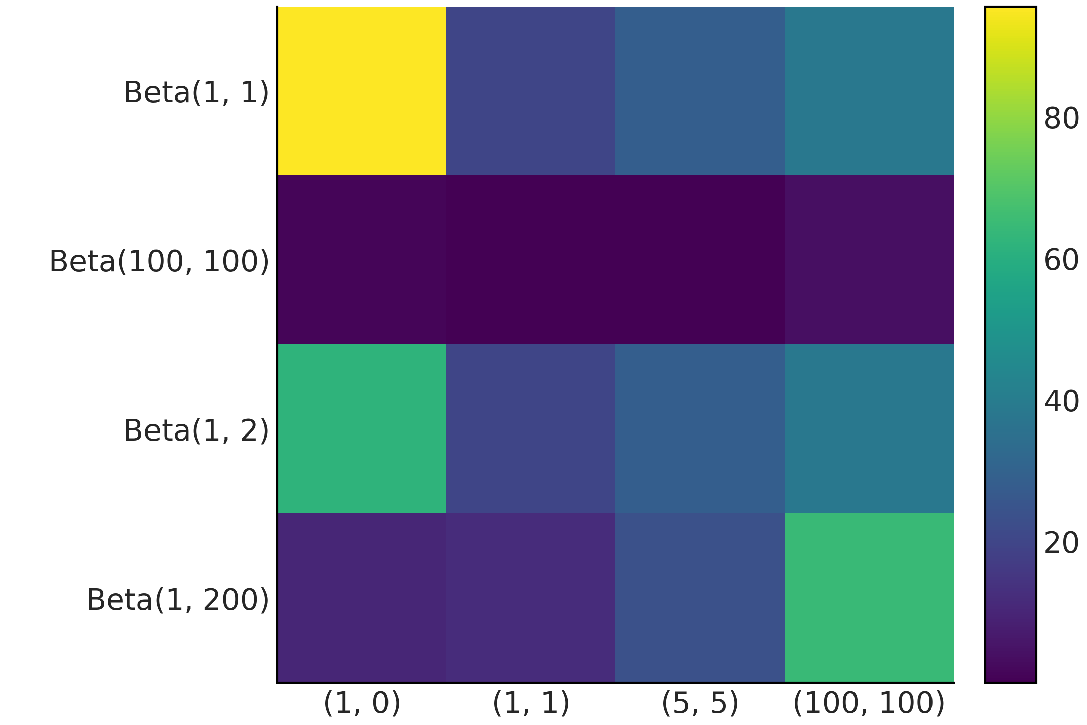
Fig. 193 热图显示使用调和平均估计器逼近 Beta-Binomial 模型的边缘似然时的相对误差。行对应于不同的先验分布。每列是不同的观测场景，括号中的数字对应于成功和失败的数量。¶

正如我们将在 11.8 走出平地部分中看到的那样，当我们增加模型的维度时，后验更多地集中在一个薄的超壳中。从这个薄壳外部获取样本与计算良好的后验近似无关。相反，当计算边缘似然时，仅从这个薄壳中获取样本是不够的。相反，我们需要对整个先验分布进行采样，而以正确的方式完成这可能是一项非常艰巨的任务。

有一些计算方法更适合计算边缘似然，但即使是那些也不是万无一失的。在第 8 章中，我们讨论了序列蒙特卡罗（SMC）方法，主要是为了进行近似贝叶斯计算，但这种方法也可以计算边缘似然。它起作用的主要原因是因为 SMC 使用一系列中间分布来表示从先验分布到后验分布的过渡。拥有这些桥接分布缓解了从广泛的先验采样和在更集中的后验进行评估的问题。

11.7.2 `边缘似然`与模型比较¶

在执行推理时，边缘似然通常被视为归一化常数，并且在计算过程中通常可以省略或取消。相反，在模型比较 [140, 141, 142] 中，边缘似然通常被视为至关重要。

为了更好地理解为什么让我们以明确表明我们的推论依赖于模型的方式编写贝叶斯定理：

\[p(\boldsymbol{\theta} \mid Y, M) = {\frac {p(Y \mid \boldsymbol{\theta}, M)\; p(\boldsymbol{\theta} \mid M)}{p(Y \mid M)}}\]

其中 \(Y\) 代表数据，\(\boldsymbol{\theta}\) 代表模型 \(M\) 中的参数。

如果我们有一组 \(k\) 模型并且我们的主要目标是只选择其中一个，我们可以选择边缘似然 \(p(Y \mid M)\) 的最大值的一个。在假设所比较的\(k\)模型的离散均匀先验分布的假设下，从贝叶斯定理中选择具有最大边缘似然的模型是完全合理的。

(110)¶\[p(M \mid Y) \propto p(Y \mid M)\; p(M)\]

如果所有模型具有相同的先验概率，则计算 \(p(Y \mid M)\) 等价于计算 \(p(M \mid Y)\)。请注意，我们讨论的是我们分配给模型 \(p(M)\) 的先验概率，而不是我们分配给每个模型 \(p(\theta \mid M)\) 参数的先验概率。

由于 \(p(Y \mid M_k)\) 的值本身并不能告诉我们任何事情，实际上人们通常会计算两个边缘似然的比率。

这个比率称为贝叶斯因子：

\[BF = \frac{p(Y \mid M_0)}{p(Y \mid M_1)}\]

\(BF > 1\) 的值表明模型 \(M_0\) 与模型 \(M_1\) 相比更能解释数据。在实践中，通常使用经验法则来指示 BF 何时小、大、不是那么大等 21。

贝叶斯因子很有吸引力，因为它是贝叶斯定理的直接应用，正如我们从公式 (110) 中看到的那样，但对于调和平均估计器也是如此（参见第 11.7.1 调和平均估计器节）和这不会自动使它成为一个好的估计器。贝叶斯因子也很有吸引力，因为与模型的似然性相反，边缘似然不一定会随着模型的复杂性而增加。直观的原因是，参数的数量越多，关于似然性的先验就越 * 散布 *。或者换句话说，一个更“分散”的先验是一个比一个更集中的数据集更合理的数据集。这将反映在边缘似然中，因为我们将在更广泛的先验比更集中的先验得到更小的值。

除了计算问题之外，边缘似然还有一个特征，它通常被认为是一个错误。它对先验的选择非常敏感。 “非常敏感”是指虽然与推理无关，但对边缘似然值有实际影响的变化。为了举例说明这一点，假设我们有模型：

(111)¶\[\begin{split}\begin{split} \mu \sim&\; \mathcal{N}(0, \sigma_0) \\ Y \sim&\; \mathcal{N}(\mu, \sigma_1) \end{split}\end{split}\]

该模型的边缘对数似然可以分析计算如下：

σ_0 = 1
σ_1 = 1
y = np.array([0])
stats.norm.logpdf(loc=0, scale=(σ_0**2 + σ_1**2)**0.5, x=y).sum()

-1.2655121234846454

如果你将先前参数 \(\sigma_0\) 的值更改为 2.5 而不是 1，边缘似然将小约 2 倍，而将其更改为 10 将小约 7 倍。你可以使用概率编程语言计算此模型的后验，并亲自了解先验在后验中的变化有多大影响。此外，你可以在下一节中检查 Fig. 194。

11.7.3 贝叶斯因子与 `WAIC` 和 `LOO`¶

在本书中，我们不使用贝叶斯因子来比较模型，而是更倾向于使用 LOO。因此，更好地理解贝叶斯因子与其他估计量的关系很有用。如果忽略细节，我们可以说：

WAIC 是后验平均的对数似然
LOO 是后验平均的对数似然
边缘似然是先验平均的（对数）似然 22。

这有助于理解三个量之间的异同。

它们都使用对数分值作为不同计算方法拟合度的度量。 WAIC 使用从后验方差计算的惩罚项。虽然 LOO 和边缘似然都避免了需要使用明确的惩罚项。 LOO 通过近似留一法交叉验证过程来实现这一点。也就是说，它使用一个数据集来拟合数据并使用不同的数据集来评估它的拟合度。边缘似然的惩罚来自对整个先验的平均，先验（相对地）到作为内置惩罚器工作的似然的传播。边缘似然中使用的惩罚似乎在某种程度上类似于 WAIC 中的惩罚，尽管 WAIC 使用后验方差，因此接近交叉验证中的惩罚。因为，如前所述，与更集中的数据集相比，更宽泛的先验承认更多的数据集是合理的，因此计算边缘似然就像对先验承认的所有数据集进行隐式平均。

概念化边缘似然的另一种等效方法是注意它是在特定数据集 \(Y\) 上评估的先验预测分布。因此，它告诉我们数据在模型下的似然有多大。该模型包括先验和似然。

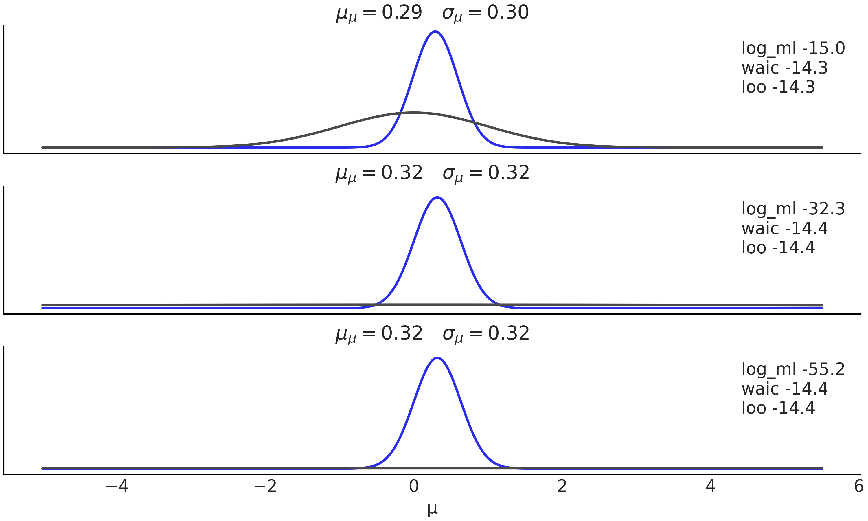
对于 WAIC 和 LOO，先验的作用是间接的。先验仅通过对后验的影响来影响 WAIC 和 LOO 的值。关于先验的数据信息越多，或者换句话说，先验和后验之间的差异越大，WAIC 和 LOO 对先验细节的敏感度就越低。相反，边缘似然直接使用先验，因为我们需要对先验的可能性进行平均。从概念上讲，我们可以说贝叶斯因子专注于识别最佳模型（并且先验是模型的一部分），而 WAIC 和 LOO 则专注于哪个（拟合）模型和参数将给出最佳预测。 Fig. 194 显示公式 (111) 中定义的模型的 3 个后验，对于 \(\sigma_0=1\)、\(\sigma_0=10\) 和 \(\sigma_0=100\)。正如我们所看到的，后验彼此非常接近，尤其是最后两个。

我们可以看到，对于不同的后验，WAIC 和 LOO 的值仅略有变化，而对数边缘似然对先验的选择很敏感。分析计算后验和对数边缘似然，WAIC 和 LOO 是从后验样本计算的（有关详细信息，请参阅随附的代码）。

Fig. 194 公式 (111) 中模型的先验（灰线）和后验（蓝线）。 WAIC 和 LOO 反映了后验分布几乎相同，而边缘似然反映了先验不同。¶

上述讨论有助于解释为什么贝叶斯因子在某些领域被广泛使用而在其他领域不受欢迎。当先验更接近反映一些潜在的真实模型时，边缘似然对先验规范的敏感性就不那么令人担忧了。当先验主要用于它们的正则化属性并且可能提供一些背景知识时，这种敏感性可能会被视为有问题。

因此，我们认为 WAIC，尤其是 LOO，具有更大的实用价值，因为它们的计算通常更健壮，并且不需要使用特殊的推理方法。在 LOO 的情况下，我们也有很好的诊断。

11.8 走出平地¶

埃德温·阿博特 [143] 的《平地：多维浪漫》中，讲述了一个生活在平地的 Square 的故事，这是一个由 \(n\) 边多边形居住的二维世界，其中状态由边数定义；女性是简单的线段，牧师坚持认为她们是圆，即使那时只是高阶多边形。这部小说于 \(1984\) 年首次出版，同样有效地讽刺了理解超出我们共同经验的想法的困难。

正如平地中的 Square 所发生的那样，我们现在要证明高维空间的怪异之处。

假设我们要估计 \(\pi\) 的值。执行此操作的简单过程如下。将一个圆刻入一个正方形，在该正方形内均匀地生成 \(N\) 个点，然后计算落在圆内的比例。从技术上讲，这是蒙特卡洛积分，因为我们正在使用（伪）随机数生成器计算定积分的值。

圆和正方形的面积与圆内的点数和总点数成正比。如果正方形的边是 \(2R\)，那么它的面积是 \((2R)^2\)，而在正方形里面的圆的面积是 \(\pi R^2\)。我们有：

\[\frac{\text{inside}}{N} \propto \frac{\pi R^2}{(2R)^2}\]

通过简化和重新排列，可以将 \(\pi\) 近似为：

\[\hat \pi = 4 \frac{\text{Count}_{inside}}{N}\]

我们可以在代码块 montecarlo 中用几行 Python 代码来实现这一点，估计值为 \(\pi\) 的模拟点和近似误差显示在 fig:monte_carlo 。

Listing 167 montecarlo¶

N = 10000
x, y = np.random.uniform(-1, 1, size=(2, N))
inside = (x**2 + y**2) <= 1
pi = inside.sum()*4/N
error = abs((pi - np.pi) / pi) * 100

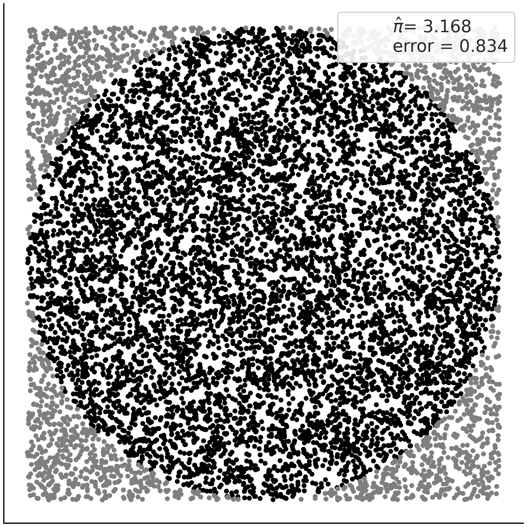
Fig. 195 使用 Monte Carlo 采样估计 \(\pi\)，图例显示了估计和百分比误差。¶

由于采样是独立同分布的，我们可以在这里应用中心极限定理，然后我们知道误差以 \(\frac{1}{\sqrt{N}}\)) 的速度减少，这意味着每增加一个小数位精度，我们需要将抽奖次数 “N” 增加 \(100\) 倍。

我们刚刚所做的是蒙特卡洛方法 23 的一个示例，基本上是任何使用（伪）随机样本来计算某些东西的方法。从技术上讲，我们所做的是蒙特卡洛积分，因为我们正在使用样本计算定积分（面积）的值。蒙特卡洛方法在统计学中无处不在。

在贝叶斯统计中，我们需要计算积分以获得后验或计算期望。你可能会建议我们可以使用这个想法的变体来计算比 \(\pi\) 更有趣的数量。

事实证明，随着我们增加问题的维度，这种方法通常不会很好地工作。在代码块 inside_out 中，我们计算从正方形采样时圆内点的数量，但从 \(2\) 到 \(15\) 维。结果在 Fig. 196 中，奇怪的是，随着增加问题的维度，即使超球体接触超立方体的壁，内部点的比例也会迅速下降。从某种意义上说，在更高维度上，超立方体的所有体积都在角落 24。

Listing 168 inside_out¶

total = 100000

dims = []
prop = []
for d in range(2, 15):
    x = np.random.random(size=(d, total))
    inside = ((x * x).sum(axis=0) < 1).sum()
    dims.append(d)
    prop.append(inside / total)

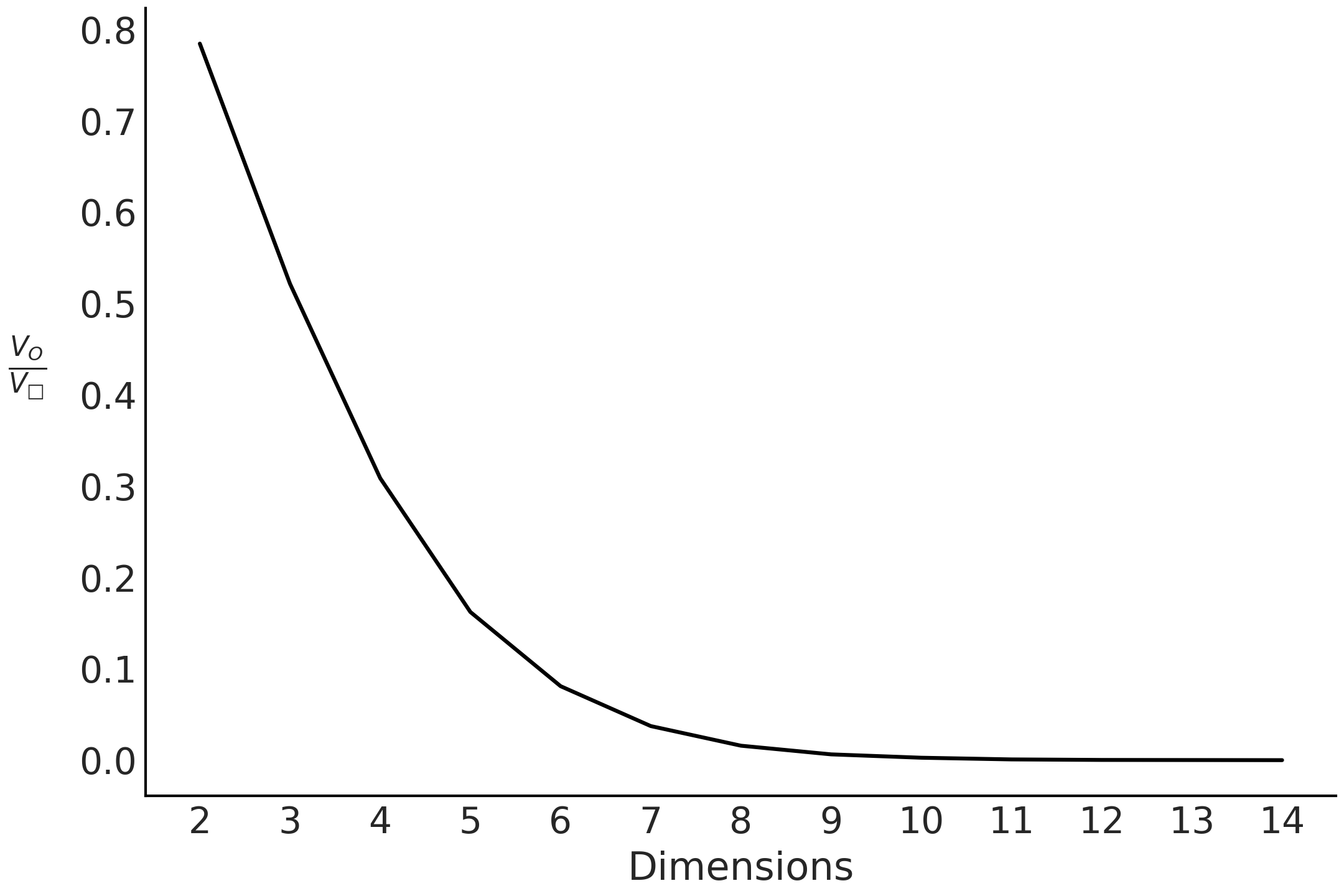
Fig. 196 当增加维度时，在超球体内获得一个点并写入超立方体的机会变为零。这表明在更高维度上，几乎所有超立方体的体积都在角落里。¶

让我们看另一个使用多元高斯的例子。Fig. 197 表明，随着增加高斯的维数，该高斯的大部分质量都位于离众数越来越远的位置。事实上，大部分质量都在众数半径 \(\sqrt{d}\) 处的一个环周围。换句话说，随着增加高斯的维数，众数变得越来越不典型。在更高的维度中，众数实际上是一个异常值，因为任何给定点在所有维度上都是众数是非常不寻常的！

我们也可以从另一个角度来看待这一点。即使在高维空间中，众数始终是密度最高的点。关键的见解是注意到它是独一无二的（就像来自平地的点！）。如果远离该众数，我们会发现单独不太可能但数量很多的点。正如在 11.1.5 连续型随机变量及其分布中看到的，概率被计算为体积上密度的积分，所以要找出分布的所有质量在哪里，必须平衡密度和体积。随着增加高斯的维度，我们最有可能从不包括该众数的环中选择一个点。

包含概率分布中大部分质量的区域被称为典型集。在贝叶斯统计中，我们非常重视它，因为如果要用样本来近似高维后验，那么样本来自典型集合就足够了。

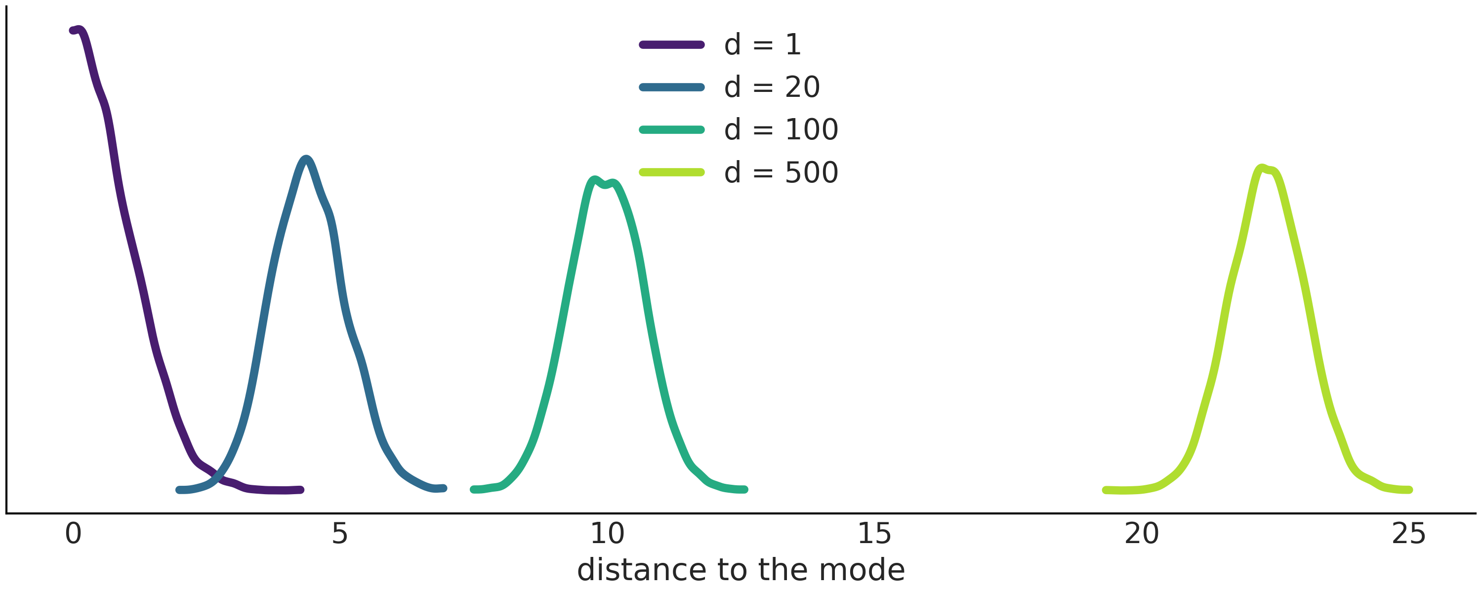
Fig. 197 当增加高斯的维度时，大部分质量分布在离该高斯众数越来越远的地方。¶

11.9 推断方法¶

有无数种计算后验的方法。如果我们在讨论共轭先验时排除在第 1 章中已经讨论过的精确解析解，则可以将推断方法分为 3 大类：

确定性集成方法。我们在书中至今尚未看到，但接下来会做；
模拟（采样）方法，在第 1 章中介绍，并贯穿全书的方法；
逼近方法，例如第 8 章中讨论的 ABC 方法，在似然函数没有封闭形式表达式的情况下使用。

虽然某些方法可能是这些类别的组合，但对可用方法进行排序还是有用的。

如果想对过去两个半世纪的贝叶斯计算方法做一个时间之旅，尤其是了解那些改变贝叶推断的方法，建议你阅读《Computing Bayes: Bayesian Computation from 1763 to the 21st Century》 [144]。

11.9.1 网格方法¶

网格方法是一种简单的蛮力方法。我们想知道后验分布在其作用域上的值以便能够使用它（找到最大值、计算期望等）。即使您无法计算整个后验，也可以逐点评估先验和似然密度函数；这是很常见的场景，即便不是最常见的场景。对于单参数模型，网格近似为：

为参数找到一个合理的区间（先验应该给出一些提示）。
在该间隔上定义一个点的网格（通常等距）。
对于网格中的每个点，将似然和先验相乘。

可选地，可以通过将每个点的结果除以所有点的总和来对计算值进行归一化，以便后验总和为 \(1\)。

代码 grid_method 计算了 Beta-Binomial 模型 的后验：

Listing 169 grid_method¶

def posterior_grid(ngrid=10, α=1, β=1, heads=6, trials=9):
    grid = np.linspace(0, 1, ngrid)
    prior = stats.beta(α, β).pdf(grid)
    likelihood = stats.binom.pmf(heads, trials, grid)
    posterior = likelihood * prior
    posterior /= posterior.sum()
    return posterior

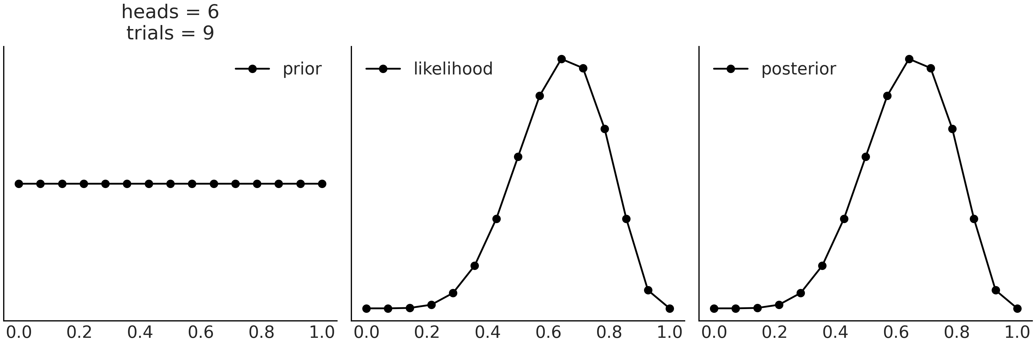
Fig. 198 通过在网格上逐点评估先验和似然，我们可以近似后验。¶

可以通过增加网格的点数来获得更好的近似值。事实上，如果使用无限数量的点，将得到精确后验，代价是需要无限的计算资源。网格方法的最大问题在于：如 {ref}high_dimensions 中所述，该方法的可扩展性随着参数数量增加会变得很差。

11.9.2 Metropolis-Hastings 采样器¶

我们很早就在第 1.2 一个自制的采样器部分介绍了 Metropolis-Hastings 算法 []，并在代码 metropolis_hastings 中展示了一个简单的 Python 实现。我们现在将提供有关此方法为何有效的更多详细信息。我们会使用第 11.1.11 马尔可夫链中介绍的马尔可夫链来完成。

Metropolis-Hastings 算法是一类通用方法，它允许我们从感兴趣的状态空间上的任何不可约马尔可夫链开始，然后将其逐步修改为具有平稳分布的新马尔可夫链。换句话说，我们从易于采样的分布（如多元正态分布）中抽取样本，并将这些样本转换为来自目标分布的样本。修改原始链的方式是有选择性的，我们只接受部分样本并拒绝其他样本。正如在 第 1 章 中看到的，接受新提议的概率为：

(112)¶\[p_a (x_{i + 1} \mid x_i) = \min \left (1, \frac{p(x_{i + 1}) \; q(x_i \mid x_{i + 1})} {p(x_i) \; q (x_{i + 1} \mid x_i)} \right)\]

让我们以更短的形式重写它，以便于操作：

\[a_{ij} = \min \left (1, \frac{p_j q_{ji}}{{p_i q_{ij}}} \right)\]

即我们以概率 \(q_{ij}\) 提议从 \(i\) 到 \(j\) 的新状态，并以概率 \(a_{ij}\) 接受该提议。这种方法的一个好处是：不需要知道待采样分布的归一化常数，因为它会在计算 \(\frac{p_j}{p_i}\) 时被消掉。这个细节非常重要，因为在许多问题中（包括贝叶斯推断），计算归一化常数都非常困难。

我们现在证明 Metropolis-Hastings 链 在平稳分布 \(p\) 下是可逆的，正如在 11.1.11 马尔可夫链节中提到的。我们需要证明细致平衡条件（即可逆性条件）成立，即：

令 \(\mathbf{T}\) 为转移矩阵，我们只需要证明所有 \(i\) 和 \(j\) 的 \(p_i t_{ij}=p_j t_{ji}\)，当 \(i=j\) 时不用讨论，所以假设 \(i \neq j\)，我们可以令：

(113)¶\[t_{ij} = q_{ij} a_{ij}\]

这意味着从 \(i\) 过渡到 \(j\) 的概率等于 “提议概率” 乘以 “接受概率”。

先看一下接受概率小于 \(1\) 的情况，此情况只发生在 \(p_j q_{ji} \le p_i q_{ij}\) 时，那么有：

(114)¶\[a_{ij} = \frac{p_j q_{ji}}{p_i q_{ij}}\]

而且

\[a_{ji} = 1\]

使用公式 (113)，有：

\[p_i t_{ij} = p_i q_{ij} a_{ij}\]

用公式 (114) 中的 \(a_{ij}\) 替换，则有：

\[p_i t_{ij} = p_i q_{ij} \frac{p_j q_{ji}}{p_i q_{ij}}\]

上述公式可简化为：

\[p_i t_{ij} = p_j q_{ji}\]

由于 \(a_{ji} = 1\) ，我们可以在不改变公式有效性的情况下包含它：

\[p_i t_{ij} = p_j q_{ji} a_{ji}\]

最终得到：

\[p_i t_{ij} = p_j t_{ji}\]

根据对称性，当 \(p_j q_{ji} > p_i q_{ij}\) 时，将得到相同的结果。因为可逆性条件成立，所以证明 \(p\) 是基于转移矩阵 \(\mathbf{T}\) 的马尔可夫链的平稳分布。

上述证明给了我们理论上的信心，即：可以使用 Metropolis-Hastings 从几乎任何分布中进行采样。还可以看到，虽然这是一个普遍结果，但它并不能帮助我们选择提议分布。因此，在实践中，提议分布的构造非常重要，并且该方法的效率在很大程度上取决于此选择。

此外，可以观察到一些普遍性规律：

如果提议发生较大的跳跃，则接受概率非常低，且大部分时间里新状态都会被拒绝，因此可能会被卡在某个地方。
如果提议的跳跃太小，则接受率很高，但探索性能变得很差，因为新状态始终位于旧状态的一个小邻域中。

因此，好的提议分布应当能够产生远离旧状态的新状态，同时又能得到很高的接受概率。

如果不知道后验分布的几何形态，通常很难做到这一点。在实践中，有用的 Metropolis-Hastings 方法通常是自适应的 []。例如：

使用多元高斯分布作为提议分布，但在调整期间，从后验样本中计算经验协方差，并将其用作提议分布的协方差矩阵；
可以缩放协方差矩阵，使平均接受率接近预定义的接受率 []等。

有证据表明，在某些情况下，当后验维度增加时，最佳接受率会收敛到神奇的数字 \(0.234\) { cite:p}Roberts1997。在实践中，\(0.234\) 左右或稍高一点的接受率或多或少会提供类似的性能，但该结果的普遍有效性和有用性存在争议 []。

在下一节中，我们将讨论一种巧妙方法来生成有助于纠正基本 Metropolis-Hastings 方法大多数问题的提议。

11.9.3 哈密顿蒙特卡洛采样器（ HMC ）¶

Hamiltonian Monte Carlo (HMC) [145, 146, 147] 是一种利用梯度生成新提议状态的 MCMC 方法。在某些状态下，后验对数概率的梯度能够提供关于后验密度函数的一些几何信息。 HMC 试图利用该梯度来提出远离当前位置且具有高接受概率的新位置，以避免典型的 Metropolis-Hastings 随机游走行为。这使得 HMC 能够更好地扩展到更高的维度，并且原则上可用于更复杂的几何形状。

简单来说，哈密顿量是对物理系统总能量的描述。我们可以将总能量分解为两个项：动能和势能。对于像滚下山这样的真实系统，势能由球的位置给出，球越高，势能越高。动能由球的速度给出，或者更准确地说是由它的动量给出（物体的速度乘以质量）。我们将假设总能量保持不变，这意味着：如果系统获得了动能，那是因为它失去了相同数量的势能。我们可以写出这样一个系统的哈密顿量为：

\[H(\mathbf{q}, \mathbf{p}) = K(\mathbf{p}, \mathbf{q}) + V(\mathbf{q})\]

其中 \(K(\mathbf{p}, \mathbf{q})\) 被称为动能，\(V(\mathbf{q})\) 为势能。在具有特定动量的特定位置找到球的概率由下式给出：

(115)¶\[p(\mathbf{q}, \mathbf{p}) = e^{-H(\mathbf{q}, \mathbf{p})}\]

为了模拟上述系统，需要求解哈密顿方程：

\[\begin{split}\begin{aligned} \frac{d \mathbf{q}}{dt} =& \quad \frac{\partial H}{\partial \mathbf{p}} = \frac{\partial K}{\partial \mathbf{p}} + \frac{\partial V}{\partial \mathbf{p}} \\ \frac{d \mathbf{p}}{dt} =& -\frac{\partial H}{\partial \mathbf{q}}= -\frac{\partial K}{\partial \mathbf{q}} - \frac{\partial V}{\partial \mathbf{q}}\end{aligned}\end{split}\]

注意：\(\frac{\partial V}{\partial \mathbf{p}} = \mathbf{0}\).

我们对从理想化的山坡上滚下理想化的球并不感兴趣，而是对沿着后验分布移动的理想化粒子建模感兴趣，为此需要进行一些调整。

首先，势能由目标分布 \(p(\mathbf{q})\) 给出；对于动量，将人为增加一个辅助变量i\(\mathbf{p}\)，或者说，一个可以帮助我们的虚构变量。如果我们选择 \(p(\mathbf{p} \mid \mathbf{q})\) ，那么可以写成：

(116)¶\[p(\mathbf{q}, \mathbf{p}) = p(\mathbf{p} | \mathbf{q}) p(\mathbf{q})\]

This ensures us that we can recover our target distribution by marginalize out the momentum. By introducing the auxiliary variable, we can keep working with the physical analogy, and later remove the auxiliary variable and go back to our problem, sampling the posterior.

这确保了我们可以通过边缘化动量来恢复目标分布。通过引入辅助变量，我们可以继续使用物理类比，然后删除辅助变量并回到我们的问题 — 对后验进行采样。如果我们将方程 canonical 替换方程 auxiliary，我们得到：

\[H(\mathbf{q}, \mathbf{p}) = \overbrace{-\log p(\mathbf{p} \mid \mathbf{q})}^{K(\mathbf{p}, \mathbf{q})} \overbrace{- \log p(\mathbf{q})}^{ + V(\mathbf{q})}\]

如前所述，势能 \(V(\mathbf{q})\) 由目标后验分布的密度函数 \(p(\mathbf{q})\) 给出，动能可以自由选择。如果选择高斯，并去掉归一化常数，则有：

\[K(\mathbf{p}, \mathbf{q}) = \frac{1}{2}\mathbf{p}^T M^{-1}\mathbf{p} + \log |M|\]

其中 \(M\) 为用于参数化高斯分布的 精度矩阵 （在哈密顿蒙特卡洛领域，也被称为 质量矩阵）。如果选择 \(M = I\)，也就是 \(n \times n\) 的单位方阵，则有：

\[K(\mathbf{p}, \mathbf{q}) = \frac{1}{2}\mathbf{p}^T \mathbf{p}\]

这使计算变得更为容易：

\[\frac{\partial K}{\partial \mathbf{p}} = \mathbf{p}\]

并且

\[\frac{\partial K}{\partial \mathbf{q}} = \mathbf{0}\]

进而，我们可以简化哈密顿方程为：

\[\begin{split}\begin{aligned} \frac{d \mathbf{q}}{dt} =& \mathbf{p} \\ \frac{d \mathbf{p}}{dt} =& - \frac{\partial V}{\partial \mathbf{q}}\end{aligned}\end{split}\]

总结起来，HMC 算法是：

获得一个 \(\mathbf{p} \sim \mathcal{N}(0, I)\) 样本
为一定量时间 \(T\) 做 \(\mathbf{q}_t\) 和 \(\mathbf{p}_t\) 模拟
\(\mathbf{q}_T\) 是提议的新状态值
使用 Metropolis 接受准则接受或者拒绝 \(\mathbf{q}_T\).

为什么我们仍然需要使用 Metropolis 验收标准？直观地说，因为我们可以将 HMC 视为具有更好提议分布的 Metropolis-Hasting 算法。但是也有一个很好的数值证明，可以表明该步骤能够纠正哈密顿方程数值模拟引入的误差。

为了计算哈密顿方程，必须计算粒子的路径，即一个状态和下一个状态之间的所有中间点。在实践中，这涉及使用积分器方法计算一系列小的积分步骤。最受欢迎的一种方法是蛙跳积分器。蛙跳积分相当于在交错的时间点更新位置 \(q_t\) 和动量 \(q_t\)，使两者交替跳过。

代码 leapfrog 展示了一个用 python 实现的蛙跳积分器 26。参数是：q 和 p 分别为初始位置和动量。 dVdq 是一个返回目标密度函数在位置 q 的梯度（ \(\frac{\part V}{\part \mathbf{q} }\) ）的 Python 函数。我们使用了 JAX [115] 的自动微分能力形成此函数。 path_len 表示积分步数，step_size 表示蛙跳步长。函数 leapfrog 输出的结果为新位置和新动量。

Listing 170 leapfrog¶

def leapfrog(q, p, dVdq, path_len, step_size):
    p -= step_size * dVdq(q) / 2  # half step
    for _ in range(int(path_len / step_size) - 1):
        q += step_size * p  # whole step
        p -= step_size * dVdq(q)  # whole step
    q += step_size * p  # whole step
    p -= step_size * dVdq(q) / 2  # half step

    return q, -p  # momentum flip at end

请注意，在函数 leapfrog 中，我们翻转了输出动量的符号。这是实现可逆 Metropolis-Hastings 提议的最简单方法，因为它通过求负步骤增加了数值积分。

我们现在拥有在 Python 中实现 HMC 方法的所有要素，如代码 hamiltonian_mc，就像我们之前在代码 metropolis_hastings 中的 Metropolis-Hasting 示例一样，这并不意味着用于严格的模型推断，而是用于演示该方法的简单示例。参数是 n_samples 为要返回的样本数，negative_log_prob 是要从中采样的负对数概率，initial_position 是开始采样的初始位置，path_len、step_size 是蛙跳参数，最终结果是我们从目标分布中获取了样本。

Listing 171 hamiltonian_mc¶

def hamiltonian_monte_carlo(
    n_samples, negative_log_prob, initial_position,
    path_len, step_size):
    # autograd magic
    dVdq = jax.grad(negative_log_prob)

    # collect all our samples in a list
    samples = [initial_position]

    # Keep a single object for momentum resampling
    momentum = stats.norm(0, 1)
    # If initial_position is a 10d vector and n_samples is 100, we want
    # 100 x 10 momentum draws. We can do this in one call to momentum.rvs, and
    # iterate over rows
    size = (n_samples,) + initial_position.shape[:1]
    for p0 in momentum.rvs(size=size):
        # Integrate over our path to get a new position and momentum
        q_new, p_new = leapfrog(
            samples[-1], p0, dVdq, path_len=path_len, step_size=step_size,
        )

        # Check Metropolis acceptance criterion
        start_log_p = negative_log_prob(samples[-1]) - np.sum(momentum.logpdf(p0))
        new_log_p = negative_log_prob(q_new) - np.sum(momentum.logpdf(p_new))
        if np.log(np.random.rand()) < start_log_p - new_log_p:
            samples.append(q_new)
        else:
            samples.append(np.copy(samples[-1]))

    return np.array(samples[1:])

Fig. 199 显示了围绕二维正态分布的三条不同的路径。对于实际采样，我们不希望路径是圆形的，因为它们会到达起始位置。相反，我们更希望从起点尽可能多地移动，例如，通过避免路径中的 \(U\) 形转弯来提高转移速度，这也就是最流行的动态 HMC 方法之一：不掉头采样 (No U-Turn Sampling, NUTS)。

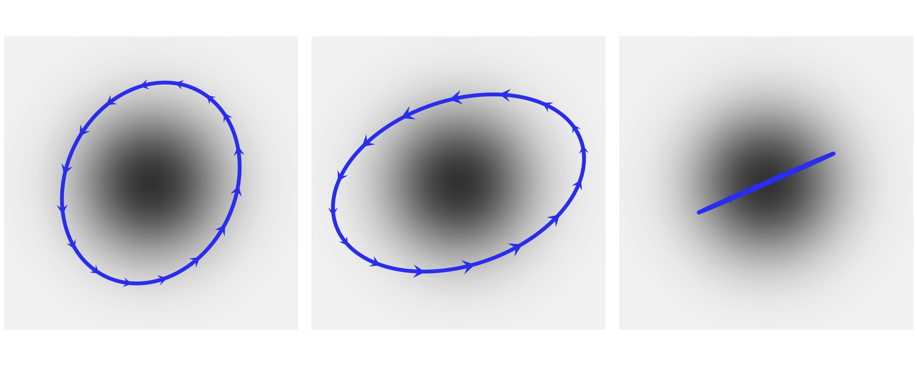
Fig. 199 Three HMC trajectories around a 2D multivariate normal. The momentum is indicated by the size and direction of the arrows, with small arrows indicating small kinetic energy. All these trajectories are computed in such a way that they end at their starting position, which completing an elliptical trajectory.¶

我们在 Fig. 200 中展示了另一个示例，它包含三条围绕同一个 Neal 漏斗的不同路径，这是我们在 4.6.2 分层模型的新问题 — 后验几何形态的复杂性带来的采样难题部分展示的（居中）分层模型中经常出现的几何形状。这是未能正确模拟遵循正确分布的路径的示例，我们将此类路径称为 发散路径，或简称为发散。如 2.4.7 散度部分所述，它们是有用的诊断。通常，像蛙跳积分器这样的辛积分器，即使对于长路径也具有很高的精度，因为它们倾向于容忍小误差并围绕正确的路径振荡。此外，这些小误差可以通过应用 Metoropolis 准则来接受或拒绝哈密顿提议以进行准确纠正。

然而，这种产生小的、易于修复的误差的能力有一个重要的例外：当精确的路径位于高曲率区域时，辛积分器生成的数值路径可能会发散，生成的路径会迅速接近目标分布的边界。

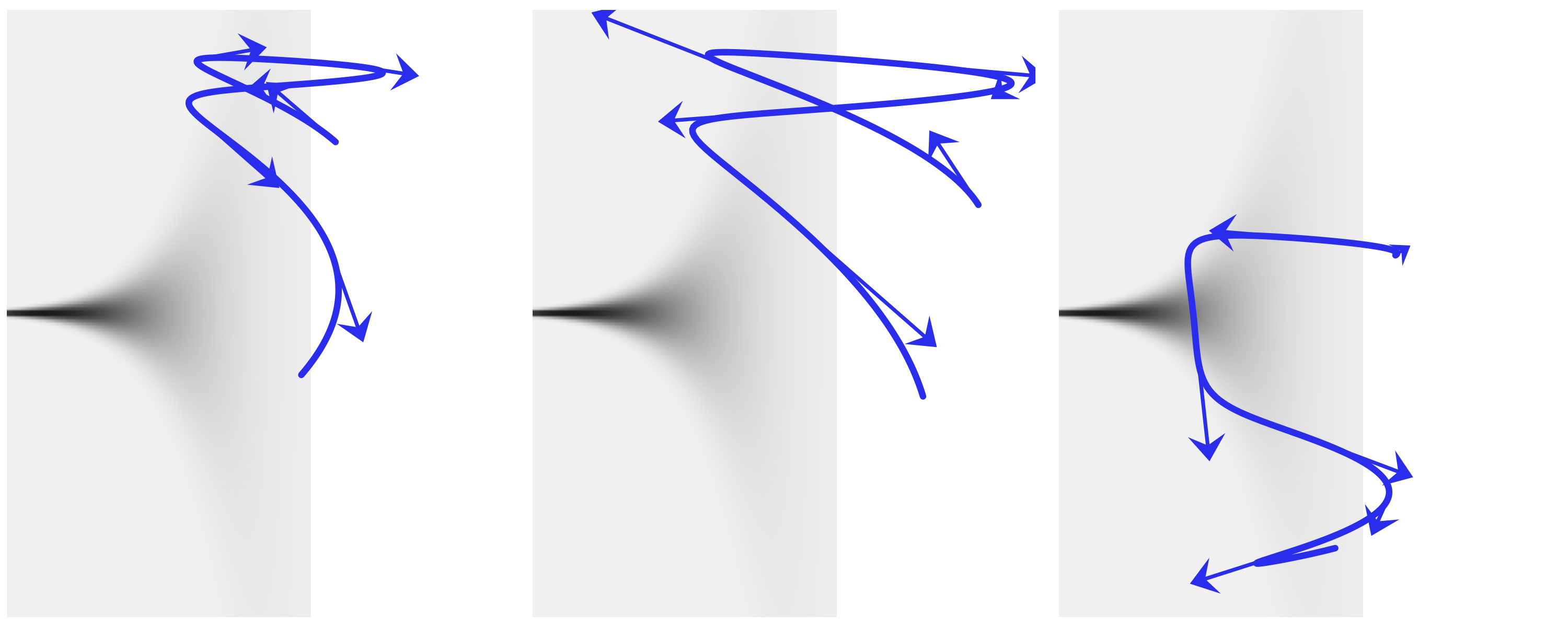
Fig. 200 Three HMC trajectories around a 2D Neal’s funnel. This kind geometry turns up in centered hierarchical models. We can see that all these trajectories when wrong. We call this kind these divergences and we can used as diagnostics of the HMC samplers.¶

图 Fig. 199 和 Fig. 200 都强调了一个事实，即有效的 HMC 方法需要适当调整其超参数。 HMC 具有三个超参数：

时间离散化（跳跃的步长）
积分时间（越级步数）
将动能参数化的精度矩阵 \(M\)

例如，如果步长太大，蛙跳积分器将不准确，并且会拒绝过多的提议。但如果它太小，将浪费计算资源。如果步数太少，每次迭代的模拟路径太短，采样会退回到随机游走。但是如果它太大，路径可能会循环运行，再次浪费计算资源。如果估计的协方差（精度矩阵的逆）与后验协方差相差太大，则提议动量将不是最优的，并且位置空间中的移动在某些维度上会太大或太小。

自适应动力学 HMC 方法，如 PyMC3、Stan 和其他 PPL 中默认使用的方法，可以在预热或调整阶段自动优化这些超参数。步长可以通过调整以匹配预定义的接受率目标来自动学习。例如，在 PyMC3 中，设置参数 target_accept 可以在预热阶段从样本中估计精度矩阵 \(M\) 或其逆矩阵，并且可以使用 NUTS 算法 在每个 MCMC 步骤动态调整步数 {cite:p }Hoffman2014。为了避免太长的路径可能会靠近初始化点，NUTS 将路径向后和向前扩展，直到满足 U 形转弯标准。此外，NUTS 应用多项式采样从路径的所有生成点中进行选择，因为这为有效探索目标分布提供了更好的准则（路径采样也可以使用固定的积分时间 HMC 完成）。

11.9.4 序贯蒙塔卡洛采样器¶

序贯蒙特卡洛（Sequential Monte Carlo,SMC ）是一系列 Monte Carlo 方法，也被称为粒子滤波器。它广泛应用于静态模型和动态模型的贝叶斯推断，例如顺序时间序列推断和信号处理 []。在相同或相似的名称下，有许多变体和实现，具有不同的应用。因此，您有时可能会发现文献有点混乱。

我们将简要描述在 PyMC3 和 TFP 中实现的 SMC/SMC-ABC 方法。有关统一框架下 SMC 方法的详细讨论，我们推荐《An Introduction to Sequential Monte Carlo》 [63]。

首先要注意，我们可以将后验写为以下形式：

\[p(\boldsymbol{\theta} \mid Y)_{\beta} \propto p(Y \mid \boldsymbol{\theta})^{\beta} \; p(\boldsymbol{\theta})\]

当 \(\beta = 0\) 时，可以看到 \(p(\boldsymbol{\theta} \mid Y)_{\beta}\) 是先验，而当 \(\beta = 1\) 时， \(p(\boldsymbol{\theta} \mid Y)_{\beta}\) 是真实后验28。

SMC 通过在 \(s\) 个连续阶段中增加 \(\beta\) 值来进行 \(\{\beta_0=0 < \beta_1 < ... < \beta_s=1\}\)。为什么这是个好主意？有两种相关的方法来证明其合理性。一是垫脚石类比。我们不是直接尝试从后验采样，而是从先验采样开始，这通常更容易做到。然后添加一些中间分布，直到到达后验（参见 Fig. 133）。二是温度类比。 \(\beta\) 参数类似于物理系统的逆温度，当我们降低它的值（增加温度），系统能够访问更多状态，当我们降低它的值（降低温度）系统 “冻结” 进入后验。Fig. 133 展示了一个假设的退火后验序列。使用温度（或其倒数）作为辅助参数被称为 回火（tempering），术语 退火（annealing） 也很常见。

在 PyMC3 和 TFP 中实现的 SMC 方法可以总结如下：

将 \(β\) 初始化为零
从回火后的后验中生成 \(N\) 个样本 \(s_β\)
增加 \(β\) 以将有效样本大小保持在预定义值
计算一组 \(N\) 个重要性权重 \(W\)。权重是根据新旧回火后验计算的
根据 \(W\) 对 \(s_β\) 重新采样得到 \(s_w\)
运行 \(N\) 个 MCMC 链 \(k\) 步，从 \(s_w\) 中的不同样本开始每个链，并仅保留最后一步中的样本
从步骤 3 重复直到 \(\beta = 1\)

重采样步骤通过删除概率低的样本并用概率较高的样本替换它们来进行。这一步降低了样本的多样性。MCMC 步骤扰动样本，希望增加多样性，从而帮助 SMC 探索参数空间。任何有效的 MCMC 转换核都可以在 SMC 中使用，并且根据问题，您可能会发现其中一些的性能优于其他核。例如，对于 ABC 方法，我们通常需要依赖无梯度方法，例如 随机游走 Metropolis-Hasting，因为模拟器通常不可微分。

回火方法的效率很大程度上取决于 \(β\) 的中间值。两个连续的 \(β\) 值之间的差异越小，两个连续的回火后验越接近，因此从一个阶段到下一个阶段的过渡越容易。但如果步骤太小，我们将需要很多中间阶段，超过某个阈值点，将浪费大量计算资源，而不能真正提高结果的准确性。另一个重要因素是增加样本多样性的 MCMC 转移核的效率。为了帮助提高转移效率，PyMC3 和 TFP 使用上一阶段的样本来调整当前阶段的提议分布以及 MCMC 采取的步骤数，并保持所有链的步数相同.

11.9.5 变分推断¶

虽然我们在本书中没有使用变分推断，但它是一种有用的方法。与 MCMC 相比，VI 往往更容易扩展到大数据并且计算运行速度更快，但收敛的理论保证较少 [148]。

正如之前在 11.3 KL 散度部分中提到的，我们可以使用一种分布来近似另一种分布，然后使用 Kullback-Leibler (KL) 散度 来衡量近似的好坏。

事实证明，我们也可以使用这种方法进行贝叶斯推理！这种方法被称为变分推理 (VI) [149]。 VI 的目标是用代理分布 \(q(θ)\) 来近似目标概率密度（在我们的例子中是后验分布 \(p(θ \mid Y)\)）。在实践中，我们通常选择 \(q(θ)\) 比 \(p(θ \mid Y)\) 具有更简单的形式，并且使用优化方法找到该分布族的具体成员，该成员在 KL 散度 意义上应当最接近目标分布。通过对方程 (96) 的微小改动，我们有：

(117)¶\[\mathbb{KL}(q(\boldsymbol{\theta}) \parallel p(\boldsymbol{\theta} \mid Y)) = \mathbb{E}_q[\log{q(\boldsymbol{\theta})}-\log{p(\boldsymbol{\theta} \mid Y)}]\]

然而，这个目标很难计算，因为它需要 \(p(Y)\) 的边缘似然。为了看到这一点，让我们展开方程 (117)：

\[\begin{split}\begin{split} \mathbb{KL}(q(\boldsymbol{\theta}) \parallel p(\boldsymbol{\theta} \mid Y)) &= \mathbb{E}[\log{q(\boldsymbol{\theta})}] - \mathbb{E}[\log{p(\boldsymbol{\theta} \mid Y)}] \\ &= \mathbb{E}[\log{q(\boldsymbol{\theta})}] - \mathbb{E}[\log{p(\boldsymbol{\theta}, Y)}] + \log{p(Y)} \end{split}\end{split}\]

幸运的是，由于 \(\log{p(Y)}\) 是关于 \(q(\boldsymbol{\theta})\) 的常数，我们可以在优化期间省略它。因此，在实践中，我们最大化 证据下界 (ELBO)，如方程 (118) 所示，这相当于最小化 KL 散度：

(118)¶\[\text{ELBO}(q) = \mathbb{E}[\log{p(\boldsymbol{\theta}, Y)}] - \mathbb{E}[\log{q(\boldsymbol{\theta})}]\]

难题的最后一块是弄清楚如何计算方程 (118) 中的期望。我们没有解决昂贵的积分问题，而是使用从代理分布 \(q(θ)\) 中抽取的 Monte Carlo 样本计算均值，并将它们插入 (118)。

变分推断的性能取决于许多因素。其中之一是选择的代理分布族。例如，更具表现力的代理分布有助于捕获目标后验分布组分之间更复杂的非线性依赖关系，因此通常会给出更好的结果（参见 Fig. 201）。

自动选择一个好的代理分布族并有效地优化它是一个活跃的研究领域。代码 vi_in_tfp 展示了在 TFP 中使用变分推断的简单示例，具有两种不同类型的代理后验分布。结果显示在 Fig. 201 中。

Listing 172 vi_in_tfp¶

tfpe = tfp.experimental
# An arbitrary density function as target
target_logprob = lambda x, y: -(1.-x)**2 - 1.5*(y - x**2)**2

# Set up two different surrogate posterior distribution
event_shape = [(), ()]  # theta is 2 scalar
mean_field_surrogate_posterior = tfpe.vi.build_affine_surrogate_posterior(
    event_shape=event_shape, operators="diag")
full_rank_surrogate_posterior = tfpe.vi.build_affine_surrogate_posterior(
    event_shape=event_shape, operators="tril")

# Optimization
losses = []
posterior_samples = []
for approx in [mean_field_surrogate_posterior, full_rank_surrogate_posterior]:
    loss = tfp.vi.fit_surrogate_posterior(
        target_logprob, approx, num_steps=100, optimizer=tf.optimizers.Adam(0.1),
        sample_size=5)
    losses.append(loss)
    # approx is a tfp distribution, we can sample from it after training
    posterior_samples.append(approx.sample(10000))

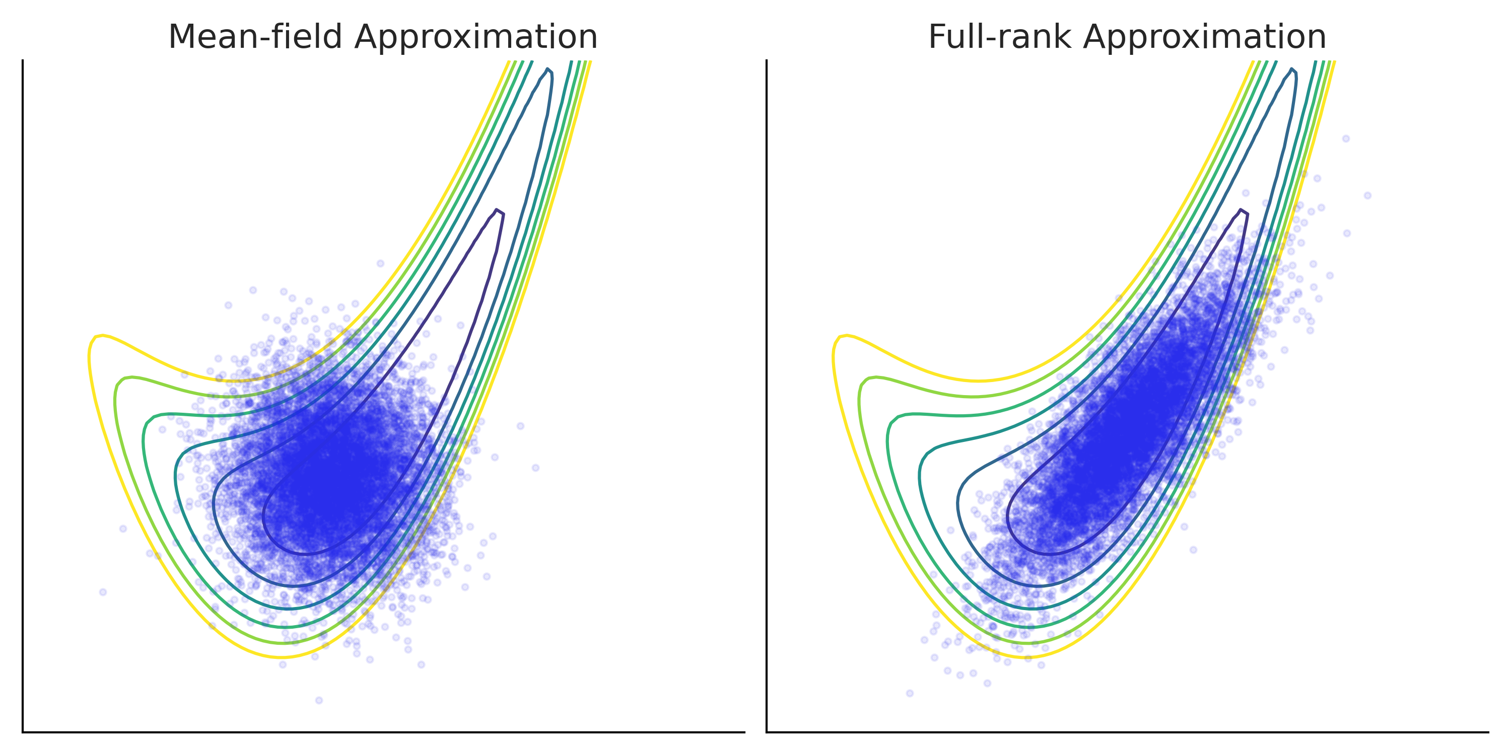
Fig. 201 Using variational inference to approximate a target density function.¶

The target density is a 2D banana shaped function plotted using contour lines. Two types of surrogate posterior distributions are used for the approximation: on the left panel a mean-field Gaussian (one univariate Gaussian for each dimension with trainable location and scale) and on the right panel a full-rank Gaussian (a 2D multivariate Gaussian with trainable mean and covariance matrix) [150].

Samples from the approximation after optimization are plotted as dots overlay on top of the true density. Comparing the two, you can see that while both approximations does not fully capture the shape of the target density, full-rank Gaussian is a better approximation thanks to its more complex structure.

11.10 编程参考¶

计算贝叶斯的一部分很好，计算机和软件工具现在可用。使用这些工具可以帮助现代贝叶斯从业者共享模型、减少错误并加快模型构建和推理过程。为了让计算机为我们工作，我们需要对其进行编程，但这通常说起来容易做起来难。要有效地使用它们仍然需要思考和理解。在最后一节中，我们将为主要概念提供一些高级指导。

11.10.1 哪种编程语言 ?¶

有许多编程语言。我们主要使用 Python，但其他流行的语言，如 Julia、R、C/C++ 也存在用于贝叶斯计算的专门应用程序。那么你应该使用哪种编程语言呢？

这里没有普遍的正确或错误答案。相反，你应该始终考虑完整的生态系统。在本书中，我们使用 Python，因为像 ArviZ、Matplotlib 和 Pandas 这样的包可以使数据处理和显示变得容易。

对于贝叶斯主义者，请特别考虑该特定语言中可用的 PPL，因为如果不存在，那么你可能需要重新考虑你选择的编程语言。还要考虑你要与之合作的社区以及他们使用的语言。

这本书的作者之一住在南加州，所以会英语和一点西班牙语很有意义，因为他可以在常见的情况下进行交流。编程语言也是如此，如果你未来的实验室组使用 R，那么学习 R 是一个好主意。

计算纯粹主义者可能会惊呼某些语言在计算上比其他语言更快。这当然是正确的，但我们建议不要过于专注于 “哪个是最快的 PPL” 的讨论。在现实生活场景中，不同模型需要不同的时间来运行。

此外，还有 “人类时间”，即迭代并提出模型的时间，以及 “模型运行时间”，即计算机返回有用结果所需的时间。这些都是不一样的，在不同的情况下，一个可能比另一个更重要。

这就是说，不要太担心选择 “正确” 的语言，如果你有效地学习了一种，概念就会转移到另一种。

11.10.2 版本控制¶

版本控制不是必需的，但绝对推荐使用，如果使用会带来很大的好处。单独工作时，版本控制可让你迭代模型设计，而不必担心丢失代码或进行更改或试验会破坏模型。这本身就可以让你更快、更有信心地进行迭代，以及在不同模型定义之间来回切换的能力。

与他人合作时，版本控制支持协作和代码共享，如果没有版本控制系统允许的快照或比较功能，这将是具有挑战性或不可能执行的。

有许多不同的版本控制系统（Mercurial、SVN、Perforce），但 git 目前是最流行的。版本控制通常不依赖于特定的编程语言。

11.10.3 依赖管理和包仓库¶

几乎所有代码都依赖于其他代码来运行。 PPL 尤其依赖于许多不同的库来运行。

我们强烈建议你熟悉一个需求管理工具，它可以帮助你查看、列出和冻结你的分析所依赖的包。此外，包存储库是从中获取这些需求包的地方。这些通常特定于该语言，例如，Python 中的一个需求管理工具是 pip，云存储库是 pypi。在 Scala 中，sbt 是一种帮助解决依赖关系的工具，而 Maven 是一种流行的包存储库。

所有成熟的语言都会有此种工具，但你必须有意识地选择使用它们。

11.10.4 环境管理¶

所有代码都在一个环境中执行。大多数人会忘记这一点，直到他们的代码突然停止工作，或者不能在另一台计算机上工作。

环境管理是用于创建可重现计算环境的一组工具。这对于在模型中处理足够随机性并且不希望计算机添加额外的可变性的贝叶斯建模者来说尤其重要。

不幸的是，环境管理也是编程中最令人困惑的部分之一。一般来说，有两种粗略的环境控制类型，语言特定的和语言不可知的。在 Python 中，virtualenv 是一个特定于 Python 的环境管理器，而容器化和虚拟化与语言无关。

我们在这里没有具体建议，因为选择很大程度上取决于你对这些工具的舒适度，以及你计划在哪里运行代码。不过，我们绝对建议你在这里做出慎重的选择，因为它可以确保你获得可重复的结果。

11.10.5 文本编辑器 vs 集成开发环境 vs Notebook¶

编写代码时，你必须将其写在某个地方。对于有数据意识的人来说，通常有三个接口。

第一个也是最简单的是文本编辑器。最基本的文本编辑器允许你惊喜地编辑文本并保存它。使用这些编辑器，你可以编写 python 程序，保存它，然后运行它。通常，文本编辑器非常 “轻量级”，除了查找和替换等基本功能之外不包含太多额外功能。把文本编辑器想象成一辆自行车。它们很简单，其界面基本上是一个车把和一些踏板，它们会让你从这里到那里，但主要是由你来完成工作。

集成开发环境 (IDE) 具有大量的功能、大量的按钮和大量的自动化。 IDE 允许你在其核心编辑文本，但顾名思义，它们也集成了开发的许多其他方面。例如，运行代码、单元测试、linting 代码、版本控制、代码版本比较等功能。在编写跨多个模块的大量复杂代码时，IDE 通常最有用。

虽然我们很乐意提供文本编辑器与 IDE 的简单定义，但如今这条线非常模糊。我们的建议是更多地从文本编辑器开始，一旦熟悉了代码的工作原理，就转向 IDE。否则，你将很难说出 IDE 在 “幕后” 为你做什么。

NoteBook 是一个完全不同的界面。其特殊之处在于混合了代码、输出和文档，并允许非线性代码执行。对于本书，大部分代码和图形都以 Jupyter Notebook 文件的形式呈现。我们还提供了 Google Colab 的链接，这是一个云笔记本环境。Notebook 通常最适合用于探索性数据分析和解释型情况，例如本书。它们不太适合运行生产代码。我们对笔记本的建议类似于 IDE。如果不熟悉统计计算，请先从文本编辑器开始。一旦你掌握了如何从单个文件运行代码，然后转移到 NoteBook 环境，无论是云托管的 Google colab、Binder 还是本地 Jupyter Notebook 。

11.10.6 本书用到的特定工具¶

这是我们用于这本书的内容。这并不意味着这些是你可以使用的唯一工具，这些只是我们使用的工具。

编程语言: Python
概率编程语言: PyMC3, TensorFlow Probability. Stan and Numpyro are displayed briefly as well.
版本控制: git
依赖管理: pip and conda
包仓库: pypi, conda-forge
环境管理: conda
通用文档: LaTeX (for book writing), Markdown (for code package), Jupyter Notebooks

参考文献¶

1: Most of the territory of what we now call Spain and Portugal was part of Al-Andalus and Arabic state, this had a tremendous influence in the Spanish/Portuguese culture, including food, music, language and also in the genetic makeup.
2: For those who are interested in delving further into the subject, we recommend reading the book Introduction to Probability by Joseph K. Blitzstein and Jessica Hwang [5].
3: From this definition John K. Kruschke wonderfully states that Bayesian inference is reallocation of credibility (probability) across possibilities [151].
4: If we need to locate the circumference relative to other objects in the plane, we would also need the coordinates of the center, but let us omit that detail for now.
5: Increase or remain constant but never decrease.
6: Loosely speaking, a right-continuous function has no jump when the limit point is approached from the right.
7: The result of one outcome does not affect the others.
8: Or more precisely if we take the limit of the Bin\((n, p)\) distribution as \(n \to \infty\) and \(p \to 0\) with \(np\) fixed we get a Poisson distribution.
9: A proper discussion that avoids non-sensical statements would require a discussion of measure theory. But we will side-step this requirement.
10: You can use check this statement yourself with the help of SciPy.
11: Not only on planet Earth, but even on other planets judging by the Gaussian-shaped UFOs we have observed (just kidding, this is of course a joke, just as ufology).
12: This distribution was discovered by William Gosset while trying to improve the methods of quality control in a brewery. Employees of that company were allow to publish scientific papers as long as they did not use the word beer, the company name, and their own surname.Thus Gosset publish under the name Student.
13: https://en.wikipedia.org/wiki/Gamma_function
14: \(\nu\) can take values below 1.
15: See, for example, https://www.youtube.com/watch?v=i5oND7rHtFs
16: For those familiar with eigenvectors and eigenvalues this should ring a bell.
17: Another analogy comes from politics, when politicians/government changes but pressing issues like inequality or climate change are not properly addressed.
18: To be precise we should include the molecules of glass and the molecules in the air, and… but let just focus on the water.
19: Do not let that Heisenberg guy and his uncertainty principle spoil the party
20: Generally pronounced as W-A-I-C, even when something like wæ[i]{.smallcaps}k is less of a mouthful
21: We do not like these rules of thumb, but you can check, for example, here https://en.wikipedia.org/wiki/Bayes_factor#Interpretation
22: In practice it is very common to actually compute the marginal likelihood in log-scale for computational stability. In such a case a Bayes factor becomes a difference of two log marginal likelihoods
23: The names derived from a famous casino with that name in the Principality of Monaco.
24: This video shows a closely related example in a very calm and clear way https://www.youtube.com/watch?v=zwAD6dRSVyI
26: Code copied from our good friend Colin Carroll’s blogpost on HMC https://colindcarroll.com/2019/04/11/hamiltonian-monte-carlo-from-scratch/
28: We mean true purely from a mathematical point of view, without any reference to how adequate is such posterior to any particular practical problem.

Bayesian Modeling and Computation in Python

第十一章：附加主题

Contents