repository open issue

Contents

第六章: 时间序列

“很难做出预测，尤其是关于未来的预测”。

据称，荷兰政治家 Karl Kristian Steincke 在 \(1940\) 年代的某个时候说过的这句话 1 。确实如此，即便今天仍然成立，特别是你在研究时间序列问题和预报问题的时候。

时间序列分析有很多应用，从面向未来的预报、到了解历史趋势中的潜在因子等。在本章中，我们将讨论涉及此问题域的一些贝叶斯方法。

• 首先，我们会将时间序列建模视为一个回归问题，从时间戳信息中解析得到设计矩阵。

• 然后，我们会探索使用自回归（Autoregressive）方法对时间相关性进行建模。

• 将上述模型进一步扩展，可以得到更具一般性的状态空间模型（ State Space Model ） 和 贝叶斯结构化时间序列模型（ Bayesian Structural Time Series model, BSTS ） ，我们将在线性高斯假设下，引入一种专门的推断方法：卡尔曼滤波器。

• 本章其余部分简要介绍了时间序列的模型比较问题，以及建模时选择先验需要考虑的因素。

6.1 时间序列问题概览

在大量现实生活的应用中，人们会按时间顺序观测数据，每次观测时都会生成时间戳。除了观测本身之外，时间戳信息在以下情况中可以提供相当丰富的信息：

• 存在一个时间趋势，例如地区人口、全球 GDP 、美国的年二氧化碳排放量等。通常这是一种整体模式，可以直观地将其标记为“增长”或“下降”。

• 有一些与时间相关的循环模式，称为季节性（ seasonality ） 2。例如，

  • 每月 温度的变化（夏季较高，冬季较低）；

  • 每月 降雨量（在世界大多数地区，冬季较低，夏季较高）；

  • 指定办公楼的 每日 咖啡消耗量（平日较高，周末减少）；

  • 每小时 的自行车租赁数量（白天比晚上多）。

• 当前数据点以某种方式提供了有关下一个数据点的信息。换句话说，**噪声( Noise )或残差( Residuals )**是相关的 3。例如，

  • 服务台的每日结案数量；

  • 股票的每日价格；

  • 每小时的温度；

  • 每小时的降雨量等。

根据上述分析，可以考虑将时间序列分解为：

(46)\[y_t = \text{Trend}_t + \text{Seasonality}_t + \text{Residuals}_t\]

大多数经典的时间序列模型都是基于此分解。在本章中，我们将讨论呈现出某种程度 时间趋势 和 季节性 的时间序列建模方法，并探索其中捕获 规则模式 和 弱规则模式 的方法。

6.2 将时间序列视为回归问题

我们将首先在一个演示数据集上，用 线性回归模型 对时间序列建模。该数据集在著名的《机器学习中的高斯过程》Rasmussen and Williams [52]一书中被用作案例。

6.2.1 简单线性回归模型

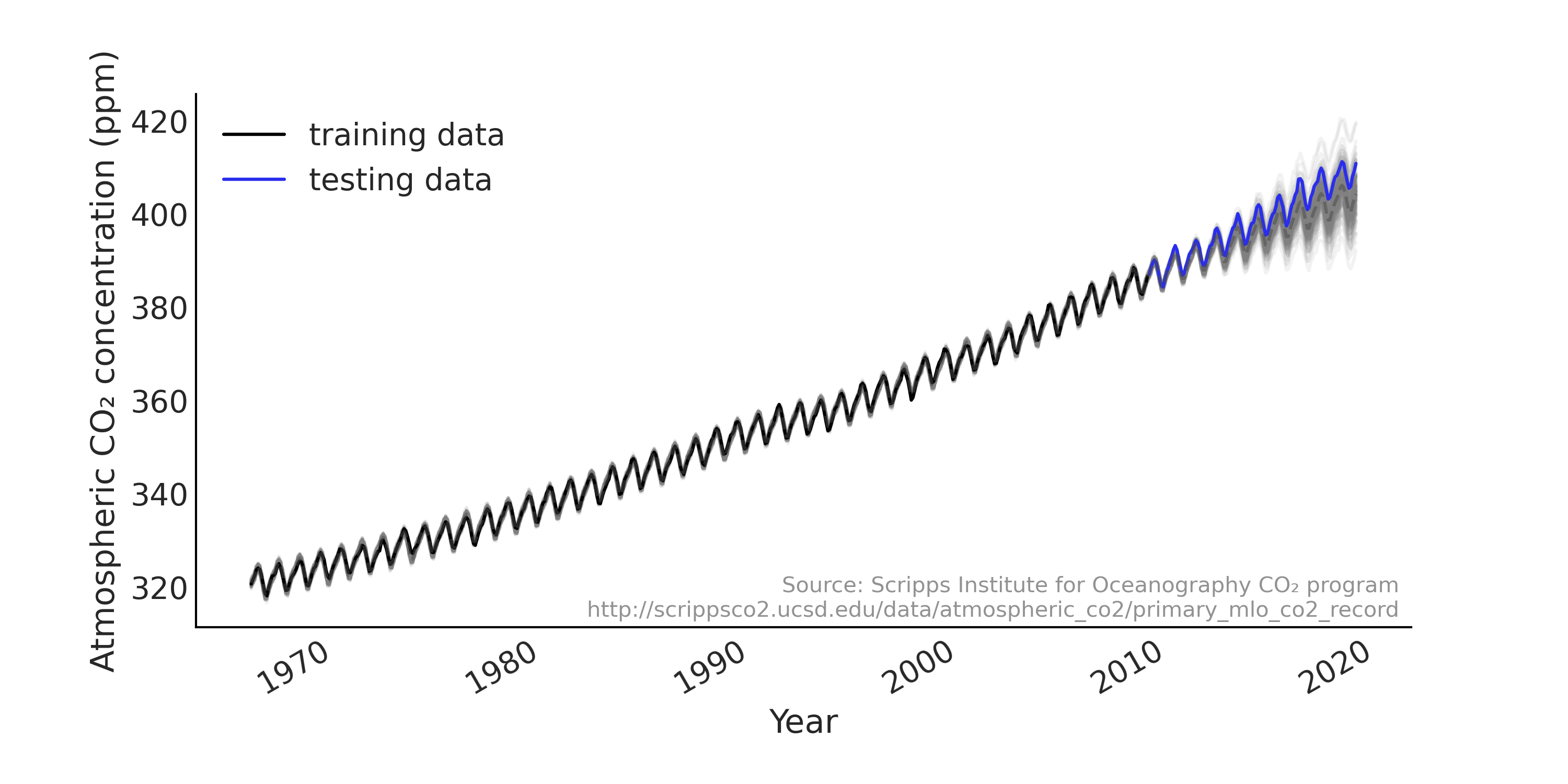
自 \(1950\) 年代后期以来，夏威夷的莫纳罗亚天文台每隔一小时就测定一次大气二氧化碳浓度。在许多示例中，该观测结果被汇总为月均值，如 Fig. 100 所示。我们使用代码 load_co2_data 将数据加载到 Python 中，然后将数据集拆分为训练集和测试集，并使用训练集拟合模型，用测试集来评估模型的预测性能。

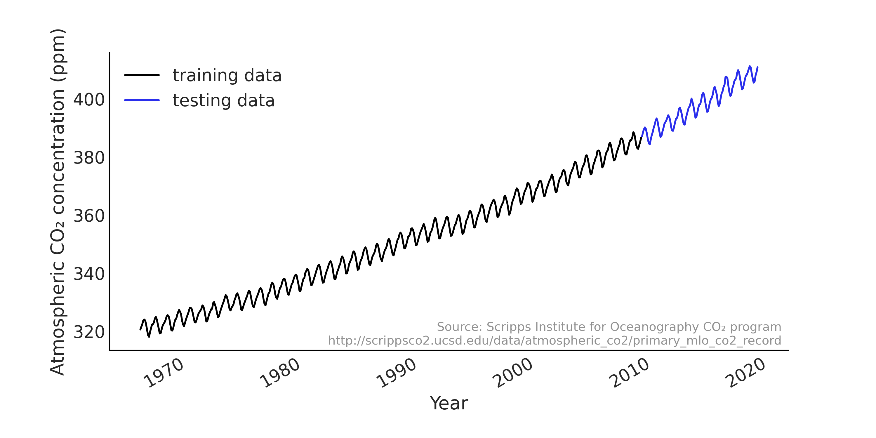
Fig. 100 从 \(1966\) 年 \(1\) 月到 \(2019\) 年 \(2\) 月，莫纳罗亚的 \(\text{CO}_2\) 月测量值，分为训练集（黑色显示）和测试集（蓝色显示）。我们可以在数据中看到强劲的上升趋势和季节性模式。

Listing 73 load_co2_data

co2_by_month = pd.read_csv("../data/monthly_mauna_loa_co2.csv")
co2_by_month["date_month"] = pd.to_datetime(co2_by_month["date_month"])
co2_by_month["CO2"] = co2_by_month["CO2"].astype(np.float32)
co2_by_month.set_index("date_month", drop=True, inplace=True)

num_forecast_steps = 12 * 10  # Forecast the final ten years, given previous data
co2_by_month_training_data = co2_by_month[:-num_forecast_steps]
co2_by_month_testing_data = co2_by_month[-num_forecast_steps:]

在这里，我们有一个每月大气 \(\text{CO}_2\) 浓度 \(y_t\) 的观测向量，其中 \(t = [0, \dots, 636]\) ；其中每个元素与一个月时间戳相关联。一年中的月份可以解析为 \([1, 2, 3,\dots, 12, 1, 2,\dots]\) 的向量。对于线性回归，可以将似然函数表述如下：

(47)\[Y \sim \mathcal{N}(\mathbf{X} \beta, \sigma)\]

考虑到季节性的影响，我们使用年预测变量的月份来索引回归系数的向量。代码 generate_design_matrix 利用独热编码将预测变量转换为 shape = (637, 12) 的设计矩阵。在该设计矩阵基础上，增加一个线性预测变量，以捕获数据中的上升趋势，进而得到整个时间序列的设计矩阵。

你可以在 Fig. 101 中看到设计矩阵的子集。

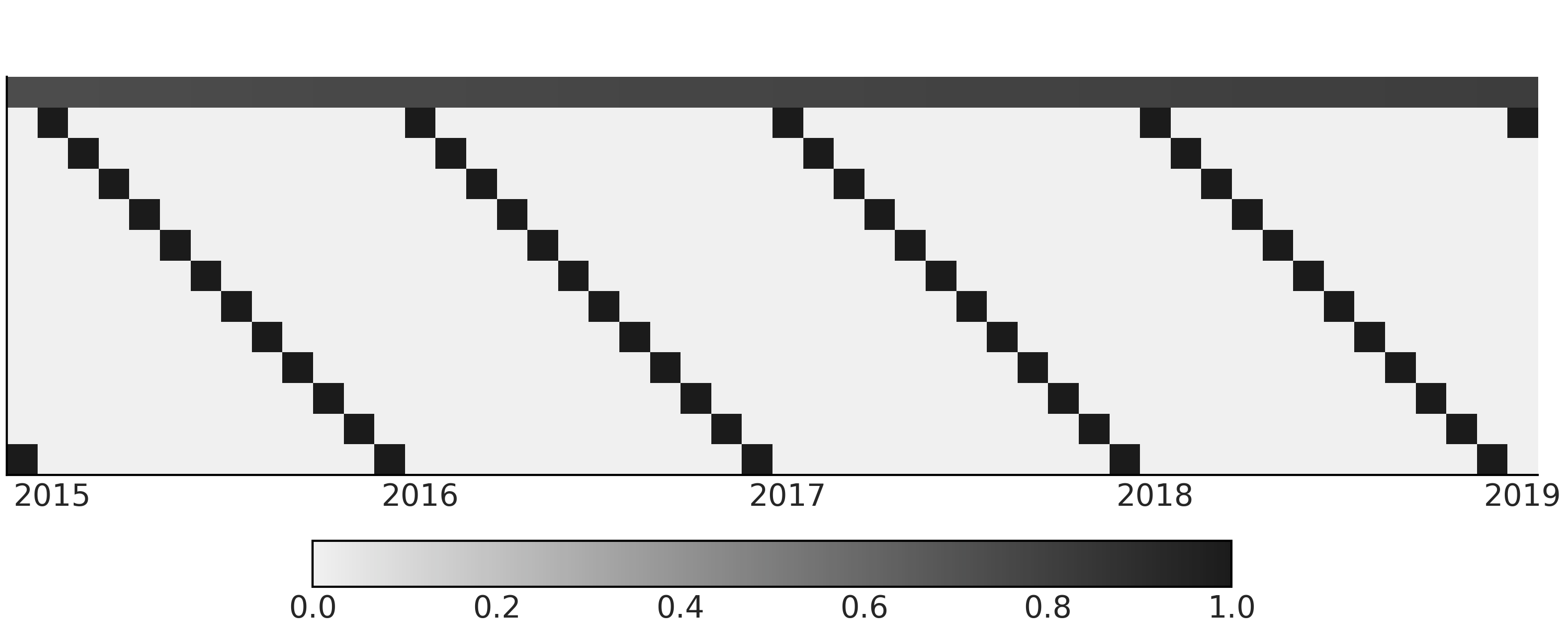
Fig. 101 为时间序列的简单回归模型提供的具有线性分量和每年各月份分量的设计矩阵。注意，真实的设计矩阵被转置成 \(feature * timestamps\) ，以便更易于可视化。图中第一行（索引 \(0\)）为 \(0\) 到 \(1\) 之间的连续值，表示时间的线性增长因子。其余行（索引 \(1 - 12\) ）为月份信息的独热编码，黑色代表 \(1\) ，浅灰色代表 \(0\) 。

Listing 74 生成设计矩阵

trend_all = np.linspace(0., 1., len(co2_by_month))[..., None]
trend_all = trend_all.astype(np.float32)
trend = trend_all[:-num_forecast_steps, :]

seasonality_all = pd.get_dummies(
   co2_by_month.index.month).values.astype(np.float32)
seasonality = seasonality_all[:-num_forecast_steps, :]

_, ax = plt.subplots(figsize=(10, 4))
X_subset = np.concatenate([trend, seasonality], axis=-1)[-50:]
ax.imshow(X_subset.T)

解析到设计矩阵的时间戳

时间戳的处理很乏味，并且容易出错，尤其是在涉及不同时区的时候。我们可以从时间戳中解析出的典型周期性信息包括（按解析顺序排列）：

• 小时的秒数 (1, 2, …, 60)

• 一天中的小时（1、2、…、24）

• 星期几（周一、周二、…、周日）

• 一个月中的某天（1、2、…、31）

• 一年中的月份（1、2、…、12）

• 节日效应（元旦、复活节、国际劳动节、圣诞节等）

所有上述信息都可以用独热编码解析为一个设计矩阵。

类似于 “一周中的某天” 和 “一个月中的某天” 等时间戳的效应通常与人类活动密切相关。例如，

• 公共交通乘客的数量通常表现出强烈的工作日效应；

• 发薪日之后，消费者支出可能会更高，这通常是在月底左右。

在本章中，我们主要考虑定期记录的时间戳。

我们现在可以使用 tfd.JointDistributionCoroutine 建立第一个面向回归问题的时间序列模型，其作法和 第 3 章 中介绍的 tfd.JointDistributionCoroutine API 和 TFP 贝叶斯建模方法相同。

Listing 75 regression_model_for_timeseries

tfd = tfp.distributions
root = tfd.JointDistributionCoroutine.Root

@tfd.JointDistributionCoroutine
def ts_regression_model():
    intercept = yield root(tfd.Normal(0., 100., name="intercept"))
    trend_coeff = yield root(tfd.Normal(0., 10., name="trend_coeff"))
    seasonality_coeff = yield root(
        tfd.Sample(tfd.Normal(0., 1.),
                   sample_shape=seasonality.shape[-1],
                   name="seasonality_coeff"))
    noise = yield root(tfd.HalfCauchy(loc=0., scale=5., name="noise_sigma"))
    y_hat = (intercept[..., None] +
             tf.einsum("ij,...->...i", trend, trend_coeff) +
             tf.einsum("ij,...j->...i", seasonality, seasonality_coeff))
    observed = yield tfd.Independent(
        tfd.Normal(y_hat, noise[..., None]),
        reinterpreted_batch_ndims=1,
        name="observed")

正如在前面章节中提到的，与 PYMC3 相比，TFP 提供了较低级别的 API 。虽然与低级模块和组件交互更灵活，但与其他概率编程语言相比，也需要更多代码，并且需要在模型中进行额外的 shape 形状处理。例如，在代码 regression_model_for_timeseries 中，我们使用 einsum 而不是 matmul 以便代码能够处理任意的 批形状（详情参阅 10.8.1 PPL 中的形状处理 ）。

代码 regression_model_for_timeseries 提供了回归模型 ts_regression_model。它具有和 tfd.Distribution 类似的功能，要抽取先验和先验预测样本，我们可以调用 .sample(.) 方法，参见代码 prior_predictive，其结果显示在 Fig. 102 中。

Listing 76 prior_predictive

# Draw 100 prior and prior predictive samples
prior_samples = ts_regression_model.sample(100)  
prior_predictive_timeseries = prior_samples.observed

fig, ax = plt.subplots(figsize=(10, 5))
ax.plot(co2_by_month.index[:-num_forecast_steps],
        tf.transpose(prior_predictive_timeseries), alpha=.5)
ax.set_xlabel("Year")
fig.autofmt_xdate()

Fig. 102 来自简单回归模型的先验预测样本，用于模拟莫纳罗亚时间序列中的月 \(\text{CO}_2\) 测量值。每条线是一个模拟的时间序列。由于使用了无信息先验，导致先验预测的结果分布范围很宽泛。

在代码 inference_of_regression_model 中，我们运行了该回归模型的推断，并将结果格式化为 az.InferenceData 对象，以便做进一步的诊断。

Listing 77 inference_of_regression_model

run_mcmc = tf.function(
    tfp.experimental.mcmc.windowed_adaptive_nuts,
    autograph=False, jit_compile=True)
mcmc_samples, sampler_stats = run_mcmc(
    1000, ts_regression_model, n_chains=4, num_adaptation_steps=1000,
    observed=co2_by_month_training_data["CO2"].values[None, ...])

regression_idata = az.from_dict(
    posterior={
        # TFP mcmc returns (num_samples, num_chains, ...), we swap
        # the first and second axis below for each RV so the shape
        # is what ArviZ expects.
        k:np.swapaxes(v.numpy(), 1, 0)
        for k, v in mcmc_samples._asdict().items()},
    sample_stats={
        k:np.swapaxes(sampler_stats[k], 1, 0)
        for k in ["target_log_prob", "diverging", "accept_ratio", "n_steps"]})

如果要依据推断结果来抽取后验预测样本，可以使用 .sample_distributions 方法先抽取后验样本，然后基于后验样本的条件化生成后验预测样本。本例中，我们还希望能够为时间序列中的 趋势性 和 季节性 分量分别抽取后验预测样本。为了可视化模型的预测能力，我们在代码 posterior_predictive_with_component 中生成了后验预测分布，结果显示在 趋势性 和 季节性 分量的后验预测分布图 Fig. 103 中，以及整体模型拟合和后验预测分布 Fig. 104 。

Listing 78 posterior_predictive_with_component

# We can draw posterior predictive sample with jd.sample_distributions()
# But since we want to also plot the posterior predictive distribution for 
# each components, conditioned on both training and testing data, we
# construct the posterior predictive distribution as below:
nchains = regression_idata.posterior.dims["chain"]

trend_posterior = mcmc_samples.intercept + \
    tf.einsum("ij,...->i...", trend_all, mcmc_samples.trend_coeff)
seasonality_posterior = tf.einsum(
    "ij,...j->i...", seasonality_all, mcmc_samples.seasonality_coeff)

y_hat = trend_posterior + seasonality_posterior
posterior_predictive_dist = tfd.Normal(y_hat, mcmc_samples.noise_sigma)
posterior_predictive_samples = posterior_predictive_dist.sample()

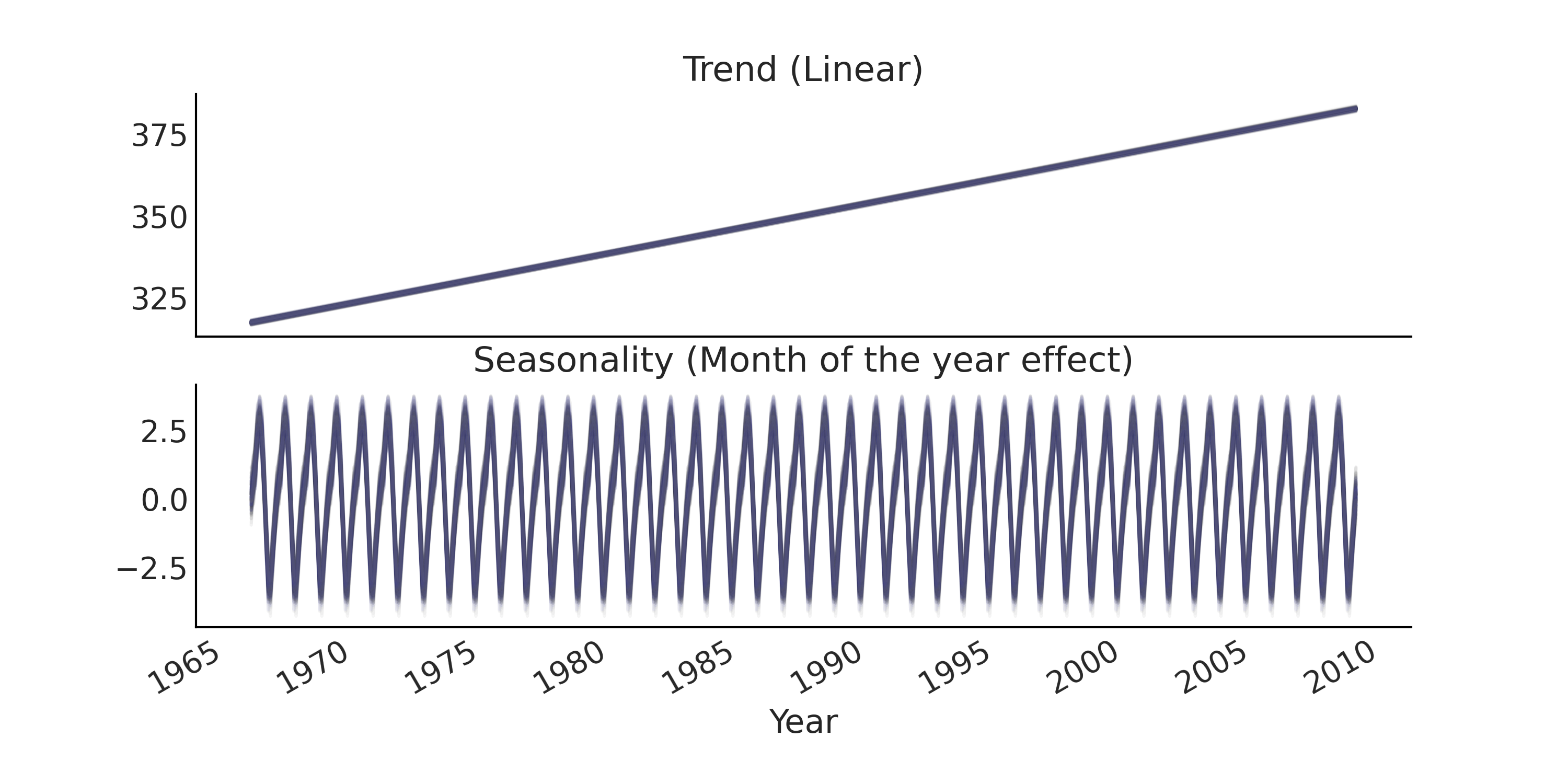
Fig. 103 时间序列回归模型的趋势性分量和季节性分量的后验预测样本。

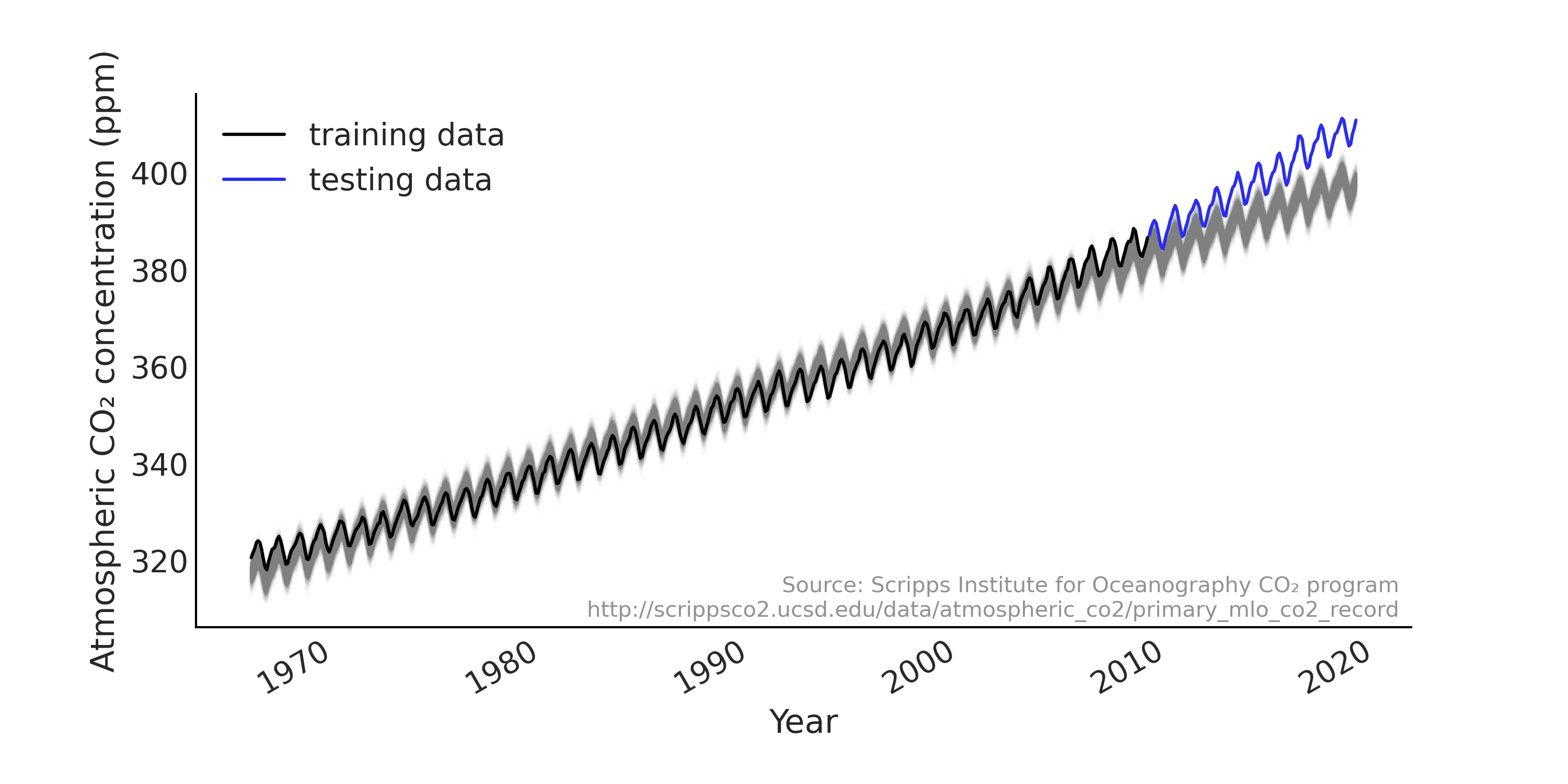
Fig. 104 时间序列简单回归模型的后验预测样本（灰色），实际数据为黑色和蓝色。虽然训练集的整体拟合（绘制为黑色）是合理的，但预测结果（样本外预测）很差，因为数据中隐含的加速趋势超出了线性关系。

查看 Fig. 104 中的样本外预测，我们注意到：

1. 当对未来预测时，线性趋势表现不佳，给出的预测始终低于实际观测值。具体来说，大气中的二氧化碳不会以恒定的斜率线性增加 4

2. 不确定性的范围几乎是恒定的，但直觉上判断，当预测更远的未来时，似乎不确定性应当增加才对（有时也称为预测锥）。

6.2.2 时间序列的设计矩阵

在上面的回归模型中，使用了一个相当简单的设计矩阵。通过向设计矩阵添加额外信息，可以获得更好的模型来捕获我们对时间序列的理解。

更好的趋势性分量模型通常是提高预测性能最重要的方面，因为相对而言，季节性分量 通常 是平稳的，具有易于估计的参数 5。因此，大多数时间序列建模都包含一个能够捕获趋势中非平稳性的隐过程（Latent Process ）。

一种非常成功的方法是对趋势性分量使用 局部线性过程 。基本上，它是一个在某个范围内呈线性的平滑趋势，模型中的截距和系数在可观测的时间跨度内缓慢变化或漂移。这种应用的一个典型例子是 Facebook Prophet 6，其中使用了 半平滑阶跃线性函数（ Semi-smooth Step Linear Function ） 对趋势进行建模 [53] 。该模型允许斜率在某些特定断点处发生变化，进而允许我们生成比直线更好的捕获长期趋势的拟合结果。这类似于在 5.2 扩展特征空间 中讨论的指示函数的想法。在时间序列场景中，我们在公式 (48) 中以数学方式表达了此想法。

(48)\[g(t) = (k + \mathbf{A}\delta) t + (m + \mathbf{A} \gamma)\]

其中 \(k\) 是（全局）增长率，\(\delta\) 是每个变化点的调整率向量，\(m\) 是（全局）截距。\(\mathbf{A}\) 是一个 shape=(n_t, n_s) 的矩阵，其中 \(n_s\) 是变化点的数量。在时间 \(t\)，\(\mathbf{A}\) 累积斜率的漂移效应 \(\delta\)。 \(\gamma\) 设置为 \(-s_j \times \delta_j\)（其中 \(s_j\) 是 \(n_s\) 个变化点的时间位置）以使趋势线连续。

通常为 \(\delta\) 选择一个正则化的先验，如 \(\text{Laplace}\)，以表示我们不希望看到斜率发生突然的或较大的变化。你可以在代码 step_linear_function_for_trend 中查看随机生成的阶跃线性函数的示例,以及在 Fig. 105 中的分解。

Listing 79 step_linear_function_for_trend

n_changepoints = 8
n_tp = 500
t = np.linspace(0, 1, n_tp)
s = np.linspace(0, 1, n_changepoints + 2)[1:-1]
A = (t[:, None] > s)

k, m = 2.5, 40
delta = np.random.laplace(.1, size=n_changepoints)
growth = (k + A @ delta) * t
offset = m + A @ (-s * delta)
trend = growth + offset

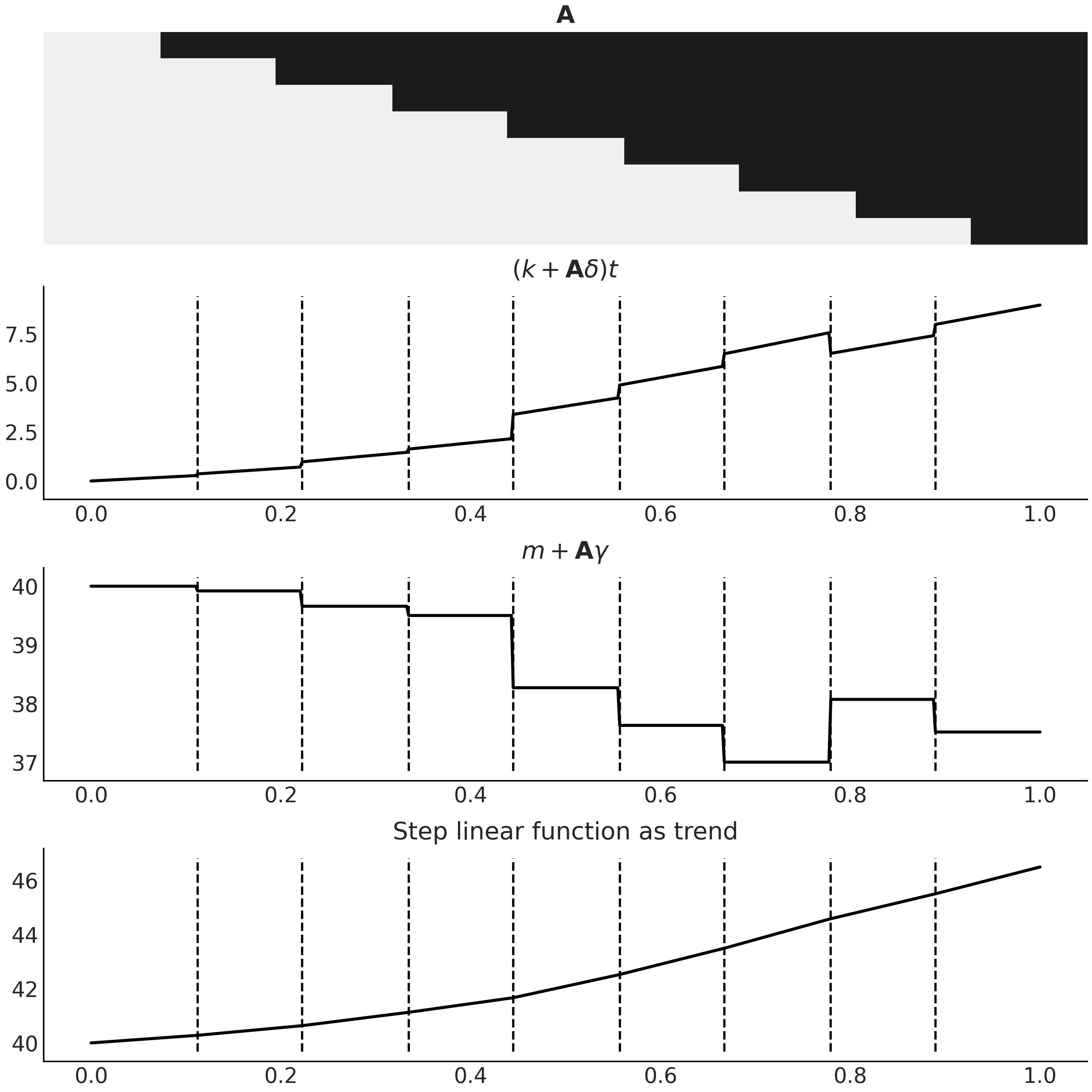
Fig. 105 作为时间序列模型趋势性分量的阶跃线性函数，使用代码 step_linear_function_for_trend 生成。第一个子图是设计矩阵 \(\mathbf{A}\)，其颜色编码相同，黑色代表 \(1\)，浅灰色代表 \(0\)。最后一个子图是公式 (48) 中可以在时间序列模型中用作趋势的结果函数 \(g(t)\) 。中间两个子图是公式 (48) 中两个分量的分解。请注意两者是如何结合使结果趋势连续的。

在实践中，我们通常会先验地指定有多少变化点，因此可以静态生成 \(\mathbf{A}\)。一种常见的方法是指定比你认为时间序列实际显示的更多的变化点，并在 \(\delta\) 上放置一个更稀疏的先验以将后验调节到 0。自动变化点检测也是可能的 [54]。

6.2.3 基函数和广义可加模型

在代码 regression_model_for_timeseries 中定义的回归模型中，我们使用了稀疏索引矩阵对季节性分量进行建模。还有一种方法是使用基样条（ 参见第 5 章 ）之类的基函数，或 Facebook Prophet 模型中的傅里叶基函数。作为设计矩阵的基函数可能会提供一些很好的属性，如正交性（参见设计矩阵的数学性质），这会使数值化求解线性公式更稳定 [55]。

傅里叶基函数是正弦和余弦函数的集合，可用于逼近任意平滑的季节性效应 [56]：

(49)\[s(t) = \sum^N_{n=1} \left[a_n \text{cos}\left(\frac{2 \pi nt}{P} \right) + b_n \text{sin}\left(\frac{2 \pi nt}{P}\right) \right]\]

其中 \(P\) 是时间序列具有的常规周期（例如，对于年度数据，\(P = 365.25\) 或对于每周数据，当时间变量以天为单位时，\(P = 7\)）。可以使用代码 fourier_basis_as_seasonality 中所示的公式静态生成它们，并在 Fig. 106 中将其可视化。

Listing 80 fourier_basis_as_seasonality

def gen_fourier_basis(t, p=365.25, n=3):
    x = 2 * np.pi * (np.arange(n) + 1) * t[:, None] / p
    return np.concatenate((np.cos(x), np.sin(x)), axis=1)

n_tp = 500
p = 12
t_monthly = np.asarray([i % p for i in range(n_tp)])
monthly_X = gen_fourier_basis(t_monthly, p=p, n=3)

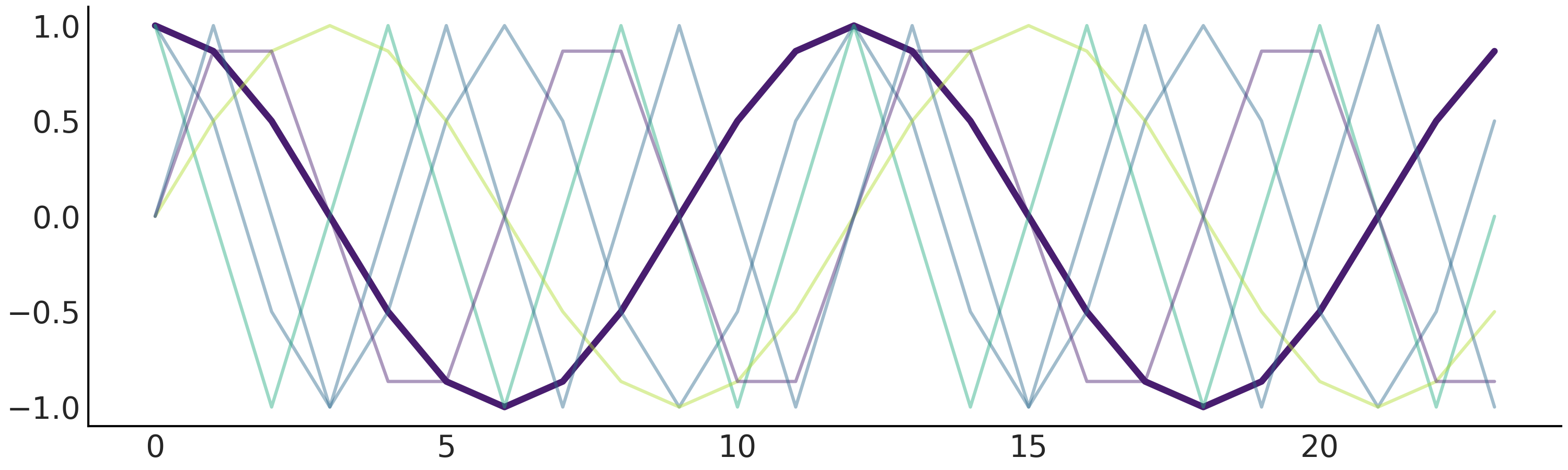
Fig. 106 \(n=3\) 的傅立叶基函数。总共有 \(6\) 个预测变量，我们通过将其余的设置为半透明来突出显示第一个。

使用上述傅里叶基函数生成的设计矩阵拟合季节性需要估计 \(2N\) 个参数 \(\beta = [a_1, b_1, \dots , a_N , b_N]\)。

像 Facebook Prophet 这样的回归模型也被称为广义可加模型 (GAM)，因为其结果变量 \(Y_t\) 线性依赖于未知的平滑基函数 7。我们之前在第 5 章中也讨论了其他 GAM。

设计矩阵的数学性质

设计矩阵的数学性质在线性最小二乘问题设置中得到了相当广泛的研究，我们想要求解 \(min \mid Y - \mathbf{X} \beta \mid ^{2}\) 的 \(\beta\)。通过检查矩阵 \(\mathbf{X}^T \mathbf{X}\) 的性质，我们通常可以了解 \(\beta\) 解的稳定程度，甚至可能得到一个解。其中一个性质是条件数，它是 \(\beta\) 的解是否容易出现较大数值误差的指示器。例如，如果设计矩阵包含高相关（多重共线性）的列，则条件数会很大，并且矩阵 \(\mathbf{X}^T \mathbf{X}\) 是病态的。类似原理也适用于贝叶斯建模。

无论你采用哪种建模方法，在分析工作流程中做深入的探索性分析都是非常有用的。基函数作为设计矩阵通常需要具备良好的条件。

用于每月二氧化碳测量结果的类 Facebook Prophet 广义可加模型见代码 gam 。我们为 k 和 m 分配了弱信息先验，以表达我们对月指标总体呈上升趋势的认知。这里得到了与实际观测非常接近的先验预测样本（参见 Fig. 107）。

Listing 81 gam

# Generate trend design matrix
n_changepoints = 12
n_tp = seasonality_all.shape[0]
t = np.linspace(0, 1, n_tp, dtype=np.float32)
s = np.linspace(0, max(t), n_changepoints + 2, dtype=np.float32)[1: -1]
A = (t[:, None] > s).astype(np.float32)
# Generate seasonality design matrix
# Set n=6 here so that there are 12 columns (same as `seasonality_all`)
X_pred = gen_fourier_basis(np.where(seasonality_all)[1],
                           p=seasonality_all.shape[-1],
                           n=6)
n_pred = X_pred.shape[-1]

@tfd.JointDistributionCoroutine
def gam():
    beta = yield root(tfd.Sample(
        tfd.Normal(0., 1.), sample_shape=n_pred, name="beta"))
    seasonality = tf.einsum("ij,...j->...i", X_pred, beta)

    k = yield root(tfd.HalfNormal(10., name="k"))
    m = yield root(tfd.Normal(
        co2_by_month_training_data["CO2"].mean(), scale=5., name="m"))
    tau = yield root(tfd.HalfNormal(10., name="tau"))
    delta = yield tfd.Sample(
        tfd.Laplace(0., tau), sample_shape=n_changepoints, name="delta")

    growth_rate = k[..., None] + tf.einsum("ij,...j->...i", A, delta)
    offset = m[..., None] + tf.einsum("ij,...j->...i", A, -s * delta)
    trend = growth_rate * t + offset

    y_hat = seasonality + trend
    y_hat = y_hat[..., :co2_by_month_training_data.shape[0]]

    noise_sigma = yield root(tfd.HalfNormal(scale=5., name="noise_sigma"))
    observed = yield tfd.Independent(
        tfd.Normal(y_hat, noise_sigma[..., None]),
        reinterpreted_batch_ndims=1,
        name="observed")

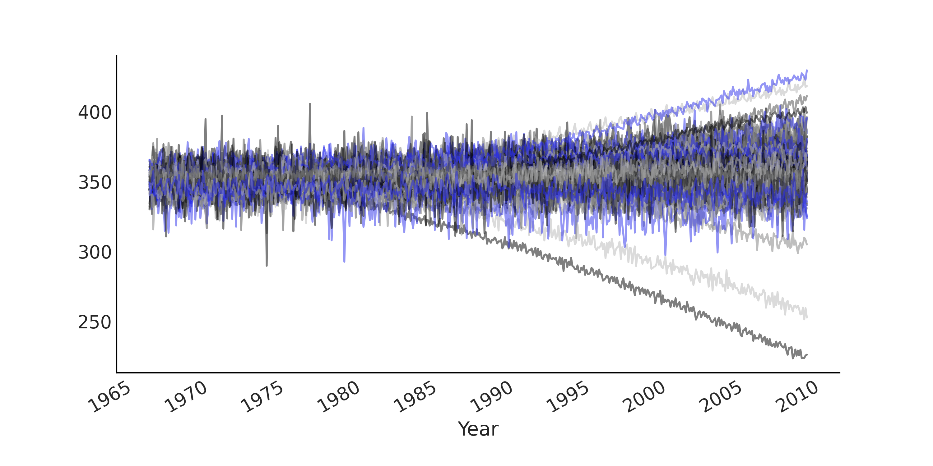
Fig. 107 从代码 gam 生成的、来自类 Facebook Prophet 广义可加模型的先验预测样本，与趋势性分量相关的参数具有弱信息先验。每条线是一个预测生成的时间序列。预测样本与实际观测值的范围相似，尤其是将此图与 Fig. 102 进行比较时更为明显。

经过推断，我们还能够得到后验预测样本，如 Fig. 108 所示，预测性能优于 Fig. 104 中的简单回归模型。

请注意，在 Taylor and Letham [53] 中，预测结果的生成过程与此处的生成模型不一样，因为阶跃线性函数被预定的变化点均匀切分开了。对于预测而言，建议在每个时间点处首先确定其是否为变化点，然后再从后验分布 \(\delta_{new} \sim \text{Laplace}(0, \tau)\) 中生成新样本。在这里，为了简化生成过程，我们简单地使用上一时段的线性趋势。

Fig. 108 来自代码 gam 的类 Facebook Prophet 模型的后验预测样本以灰色显示，实际数据以黑色和蓝色显示。

6.3 自回归模型

6.3.1 基础的自回归模型

时间序列的特征之一是观测值之间存在顺序依赖性。这通常会引入与先前观测（或观测误差）相关的结构化误差，其中典型的是自回归性。在自回归模型中，时间 \(t\) 处的分布被先前观测值的线性函数参数化。考虑一个具有高斯似然的一阶自回归模型（ 通常记作 \(AR(1)\) ）：

(50)\[y_t \sim \mathcal{N}(\alpha + \rho y_{t-1}, \sigma)\]

\(y_t\) 遵循在该位置处的高斯分布，并且是 \(y_{t-1}\) 的线性函数。

（ 1 ）采用循环语句实现自回归

在 Python 中，可以用一个 for 循环来编写这样一个自回归模型。例如，在代码 ar1_with_forloop 中，我们使用 \(\alpha = 0\) 的 tfd.JointDistributionCoroutine 创建了一个 \(AR(1)\) 过程，并以 \(\sigma = 1\) 和 不同的 \(\rho\) 值做条件化抽取了随机样本，其结果显示在 Fig. 109 中。

Listing 82 ar1_with_forloop

n_t = 200

@tfd.JointDistributionCoroutine
def ar1_with_forloop():
    sigma = yield root(tfd.HalfNormal(1.))
    rho = yield root(tfd.Uniform(-1., 1.))
    x0 = yield tfd.Normal(0., sigma)
    x = [x0]
    for i in range(1, n_t):
        x_i = yield tfd.Normal(x[i-1] * rho, sigma)
        x.append(x_i)

nplot = 4
fig, axes = plt.subplots(nplot, 1)
for ax, rho in zip(axes, np.linspace(-1.01, 1.01, nplot)):
    test_samples = ar1_with_forloop.sample(value=(1., rho))
    ar1_samples = tf.stack(test_samples[2:])
    ax.plot(ar1_samples, alpha=.5, label=r"$\rho$=%.2f" % rho)
    ax.legend(bbox_to_anchor=(1, 1), loc="upper left",
              borderaxespad=0., fontsize=10)

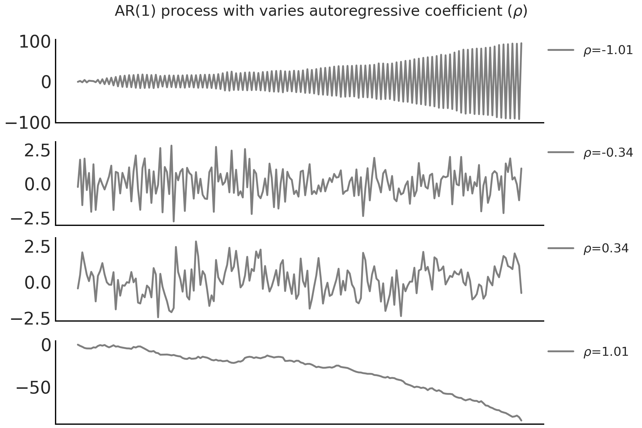
Fig. 109 \(\sigma = 1\) 和不同 \(\rho\) 值时 \(AR(1)\) 自回归过程的随机样本。请注意，当 \(\mid \rho \mid > 1\) 时，\(AR(1)\) 过程是非平稳的。

（ 2 ）使用向量化实现自回归

使用 for 循环生成时间序列随机变量非常简单，但现在每个时间点都是一个随机变量，其应用起来非常困难（ 例如，难以适应大规模的时间点数据 ）。如果可能，我们更喜欢编写使用向量化操作的模型。上面的模型可以在不使用 for 循环的情况下，通过 TFP 中的自回归分布 tfd.Autoregressive 来重写。它采用distribution_fn 函数来定义公式 (50) ，该函数输入 \(y_{t -1}\) 并返回 \(y_t\) 的分布。但 TFP 中的自回归分布仅保留了过程的最终状态，即初始值 \(y_0\) 迭代 \(t\) 步后，随机变量 \(y_t\) 的分布。为了获得自回归过程中的所有时间步，需要使用后移运算符（也称为滞后运算符）\(\mathbf{B}\) 表达公式 (50)，该运算符会对时间序列中所有 \(t > 0\) 做移动，使得 \(\mathbf{B} y_t = y_{t-1}\) 。用后移运算符 \(\mathbf{B}\) 重新表示公式 (50) 为 \(Y \sim \mathcal{N}(\rho \mathbf{B} Y, \sigma)\) 。从概念上讲，可以将其视为对向量化似然 Normal(ρ * y[:-1], σ).log_prob(y[1:]) 的估计。在代码 ar1_without_forloop 中，我们用 tfd.Autoregressive API 构建了步数为 n_t 的同一生成式 \(AR(1)\) 模型。请注意，在代码 ar1_without_forloop 中并没有通过生成输出结果 \(y_{t-1}\) 来显式地构造后移运算符 \(\mathbf{B}\) ，而是使用了 Python 函数 ar1_fun 完成后移运算并为下一时间步生成分布。

Listing 83 ar1_without_forloop

@tfd.JointDistributionCoroutine
def ar1_without_forloop():
    sigma = yield root(tfd.HalfNormal(1.))
    rho = yield root(tfd.Uniform(-1., 1.))

    def ar1_fun(x):
        # We apply the backshift operation here
        x_tm1 = tf.concat([tf.zeros_like(x[..., :1]), x[..., :-1]], axis=-1)
        loc = x_tm1 * rho[..., None]
        return tfd.Independent(tfd.Normal(loc=loc, scale=sigma[..., None]),
                               reinterpreted_batch_ndims=1)

    dist = yield tfd.Autoregressive(
        distribution_fn=ar1_fun,
        sample0=tf.zeros([n_t], dtype=rho.dtype),
        num_steps=n_t)

现在以 \(AR(1)\) 过程作为似然函数来扩展上述 类 Facebook Prophet 的广义可加模型。但需要先将代码 gam 中的 GAM 改写为代码 gam_alternative。

Listing 84 gam_alternative

def gam_trend_seasonality():
    beta = yield root(tfd.Sample(
        tfd.Normal(0., 1.), sample_shape=n_pred, name="beta"))
    seasonality = tf.einsum("ij,...j->...i", X_pred, beta)

    k = yield root(tfd.HalfNormal(10., name="k"))
    m = yield root(tfd.Normal(
        co2_by_month_training_data["CO2"].mean(), scale=5., name="m"))
    tau = yield root(tfd.HalfNormal(10., name="tau"))
    delta = yield tfd.Sample(
        tfd.Laplace(0., tau), sample_shape=n_changepoints, name="delta")

    growth_rate = k[..., None] + tf.einsum("ij,...j->...i", A, delta)
    offset = m[..., None] + tf.einsum("ij,...j->...i", A, -s * delta)
    trend = growth_rate * t + offset
    noise_sigma = yield root(tfd.HalfNormal(scale=5., name="noise_sigma"))
    return seasonality, trend, noise_sigma

def generate_gam(training=True):

    @tfd.JointDistributionCoroutine
    def gam():
        seasonality, trend, noise_sigma = yield from gam_trend_seasonality()
        y_hat = seasonality + trend
        if training:
            y_hat = y_hat[..., :co2_by_month_training_data.shape[0]]

        # likelihood
        observed = yield tfd.Independent(
            tfd.Normal(y_hat, noise_sigma[..., None]),
            reinterpreted_batch_ndims=1,
            name="observed"
        )

    return gam

gam = generate_gam()

比较代码 gam_alternative 和代码 gam，可以看到两个主要区别：

1. 将趋势性分量和季节性分量（及其先验）的构造拆分成了独立函数，并且在 tfd.JointDistributionCoroutine 的模型块中，使用了 yield from 语句，从而在不同代码中能够获得相同的 tfd.JointDistributionCoroutine 模型；

2. 将 tfd.JointDistributionCoroutine 封装在另一个 Python 函数中，这样更容易在训练集和测试集上进行条件化。

代码 gam_alternative 是一种更加模块化的方法。我们可以通过改变似然部分来写出一个具有 \(AR(1)\) 似然的 GAM 。这正是代码 gam_with_ar_likelihood 所做的。

Listing 85 gam_with_ar_likelihood

def generate_gam_ar_likelihood(training=True):

    @tfd.JointDistributionCoroutine
    def gam_with_ar_likelihood():
        seasonality, trend, noise_sigma = yield from gam_trend_seasonality()
        y_hat = seasonality + trend
        if training:
            y_hat = y_hat[..., :co2_by_month_training_data.shape[0]]

        # Likelihood
        rho = yield root(tfd.Uniform(-1., 1., name="rho"))
        def ar_fun(y):
            loc = tf.concat([tf.zeros_like(y[..., :1]), y[..., :-1]],
                            axis=-1) * rho[..., None] + y_hat
            return tfd.Independent(
                tfd.Normal(loc=loc, scale=noise_sigma[..., None]),
                reinterpreted_batch_ndims=1)
        observed = yield tfd.Autoregressive(
            distribution_fn=ar_fun,
            sample0=tf.zeros_like(y_hat),
            num_steps=1,
            name="observed")

    return gam_with_ar_likelihood

gam_with_ar_likelihood = generate_gam_ar_likelihood()

（3）通过修改设计矩阵实现自回归

另外一种实现 \(AR(1)\) 模型方法，是将线性回归概念扩展为在设计矩阵中包含一个观测相关列，并将该列的元素 \(x_i\) 设置为 \(y_{i-1}\)。然后，自回归系数 \(\rho\) 与任何其他回归系数没有什么不同，这只是告诉我们，先前观测对当前观测的期望的线性贡献是什么 8。在这个模型中，检查 \(\rho\) 的后验分布后，我们发现这种影响几乎可以忽略不计（ 参见 Fig. 110 ）：

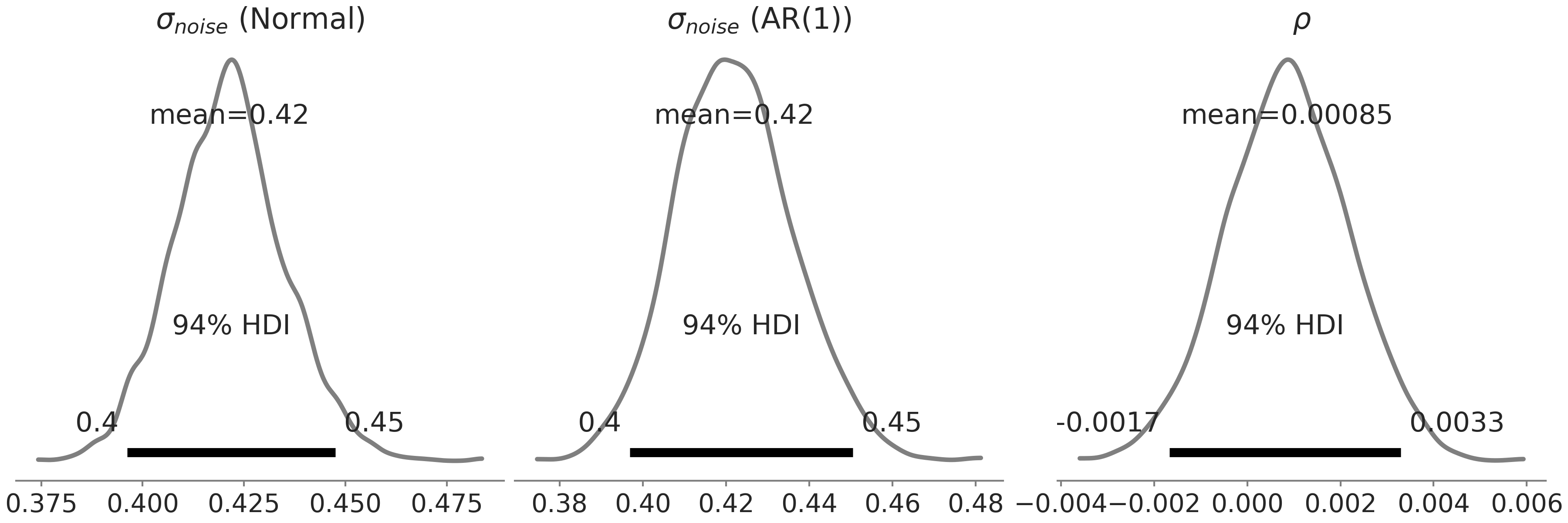
Fig. 110 在代码 gam_with_ar_likelihood 中定义的 类 Facebook Prophet 似然函数参数的后验分布。最左边的子图是具有高斯似然的模型中的 \(\sigma\)，中间和最右边的子图是具有 \(AR(1)\) 似然的模型中的 \(\sigma\) 和 \(\rho\)。两个模型都返回了相似的 \(\sigma\) 估计值，\(\rho\) 估计值以 \(0\) 为中心。

（ 4 ）隐自回归分量的引入

除了采用 AR(k) 似然函数这种方式之外，还可以在线性预测中添加隐自回归分量，来达到将自回归包含在时间序列模型中的目的。这就是代码 gam_with_latent_ar 中的 gam_with_latent_ar 隐自回归模型。

Listing 86 gam_with_latent_ar

def generate_gam_ar_latent(training=True):

    @tfd.JointDistributionCoroutine
    def gam_with_latent_ar():
        seasonality, trend, noise_sigma = yield from gam_trend_seasonality()
        
        # Latent AR(1)
        ar_sigma = yield root(tfd.HalfNormal(.1, name="ar_sigma"))
        rho = yield root(tfd.Uniform(-1., 1., name="rho"))
        def ar_fun(y):
            loc = tf.concat([tf.zeros_like(y[..., :1]), y[..., :-1]],
                            axis=-1) * rho[..., None]
            return tfd.Independent(
                tfd.Normal(loc=loc, scale=ar_sigma[..., None]),
                reinterpreted_batch_ndims=1)
        temporal_error = yield tfd.Autoregressive(
            distribution_fn=ar_fun,
            sample0=tf.zeros_like(trend),
            num_steps=trend.shape[-1],
            name="temporal_error")

        # Linear prediction
        y_hat = seasonality + trend + temporal_error
        if training:
            y_hat = y_hat[..., :co2_by_month_training_data.shape[0]]

        # Likelihood
        observed = yield tfd.Independent(
            tfd.Normal(y_hat, noise_sigma[..., None]),
            reinterpreted_batch_ndims=1,
            name="observed"
        )

    return gam_with_latent_ar

gam_with_latent_ar = generate_gam_ar_latent()

通过显式的隐自回归过程，我们在模型中添加到一个与观测数据集大小相同的随机变量。由于它现在是添加到线性预测 \(\hat{Y}\) 中的显式分量，因此可以将自回归过程解释对趋势性分量的补充，或者解释为趋势性分量的一部分。

我们可以在完成推断后，可视化隐自回归分量，类似于时间序列模型的趋势性分量和季节性分量（参见 Fig. 111）。

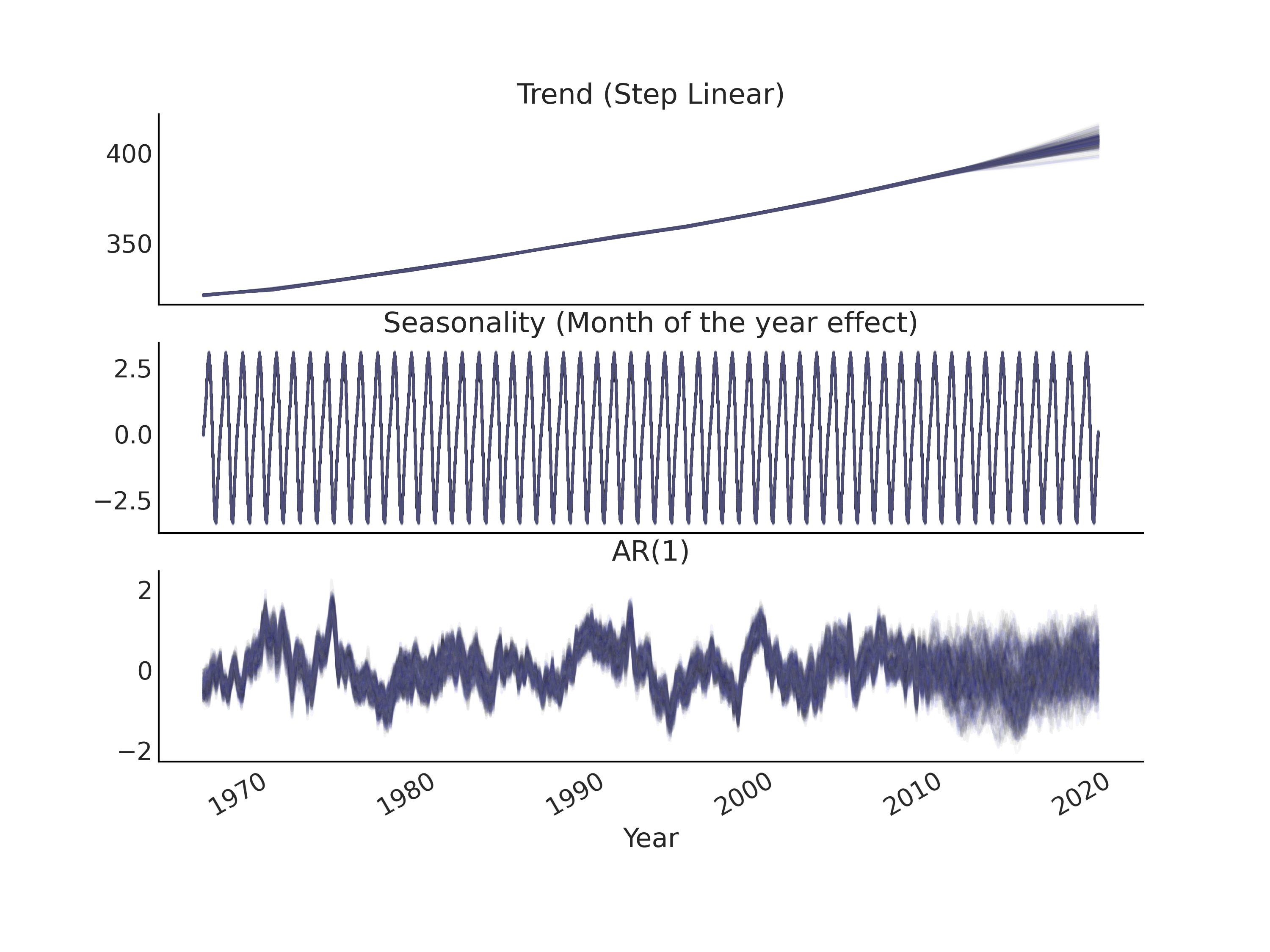
Fig. 111 在代码 gam_with_latent_ar 中指定的时间序列模型 gam_with_latent_ar 中，趋势性分量、季节性分量和 \(AR(1)\) 分量的后验预测样本。

还有一种解释隐自回归过程的方法，即认为它捕获了和时间相关的残差，因此我们预期 \(\sigma_{noise}\) 的后验估计会比没有隐自回归过程分量时的模型小。在 Fig. 112 中，我们展示了模型 gam_with_latent_ar 的 \(\sigma_{noise}\)、\(\sigma_{AR}\) 和 \(\rho\) 的后验分布。与模型 gam_with_ar_likelihood 相比，确实得到了 \(\sigma_{noise}\) 的较低估计，而 \(\rho\) 的估计则明显更高一些。

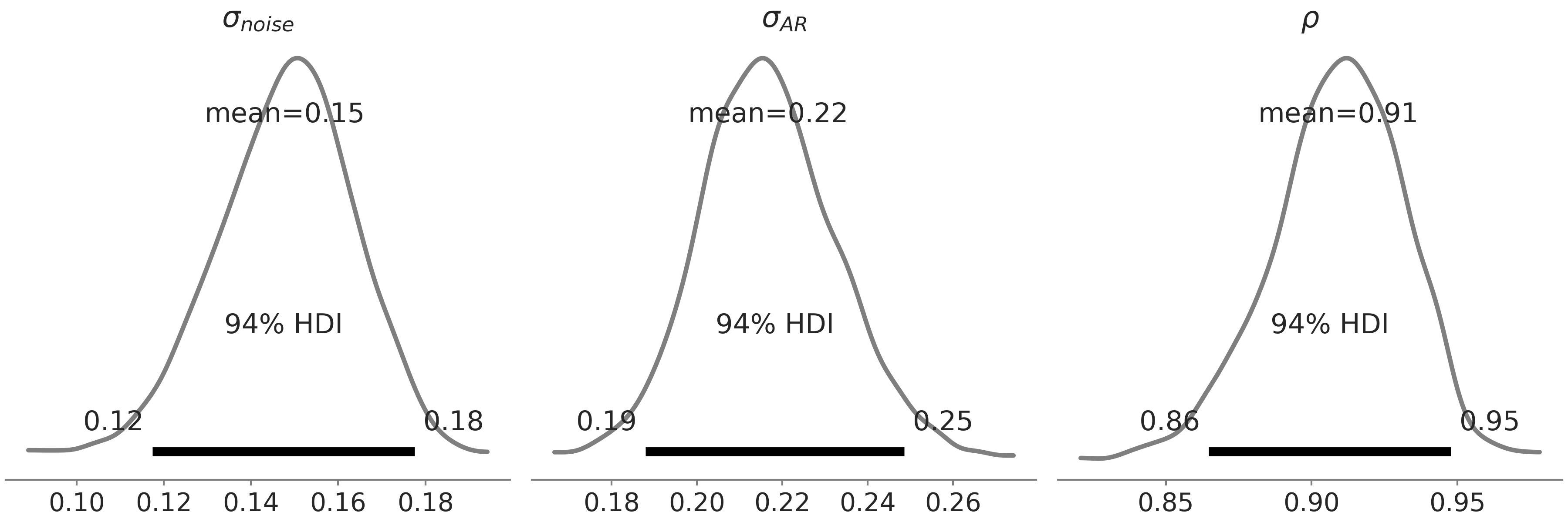
Fig. 112 代码 gam_with_latent_ar 指定的 gam_with_latent_ar 模型中， \(AR(1)\) 分量的 \(\sigma_{noise}\)、\(\sigma_{AR}\) 和 \(\rho\) 的后验分布。注意不要与 Fig. 110 混淆，在那幅图中，我们展示了来自 \(2\) 个不同 GAM 模型的参数的后验分布。

6.3.2 隐自回归过程和平滑

隐过程在捕获时间观测序列中的微妙趋势方面非常强大。它甚至可以近似任意的函数。为了证明这一点，让我们考虑使用一个包含隐高斯随机游走分量（ GRW ）的时间序列模型，对玩具数据集进行建模，如公式 (51) 所示。

(51)\[\begin{split}\begin{split} z_i & \sim \mathcal{N}(z_{i-1}, \sigma_{z}^2) \: \text{ for } i=1,\dots,N \\ y_i & \sim \mathcal{N}(z_i, \sigma_{y}^2) \end{split}\end{split}\]

此处的高斯随机游走等同于 \(\rho = 1\) 时的 \(AR(1)\) 过程。

通过在公式 (51) 中对 \(\sigma_{z}\) 和 \(\sigma_{y}\) 设置不同先验，可以突出表达高斯随机游走应当解释多少观测数据中的方差，以及其中有多少是独立同分布的噪声。我们还可以计算一个位于 \([0, 1]\) 区间内的比率值 \(\alpha = \frac{\sigma_{y}^2}{\sigma_{z}^2 + \sigma_{y}^2}\) ，并将其解释为平滑度。因此，可以将公式 (51) 中的模型等价地表示为公式 (52)。

(52)\[\begin{split}\begin{split} z_i & \sim \mathcal{N}(z_{i-1}, (1 - \alpha) \sigma^2) \: \text{ for } i=1,\dots,N \\ y_i & \sim \mathcal{N}(z_i, \alpha \sigma^2) \end{split}\end{split}\]

公式 (52) 中的隐高斯随机游走模型可以编写为代码 gw_tfp 。通过在 \(\alpha\) 上放置信息性先验，我们可以控制希望在隐高斯随机游走分量中看到多少平滑度， \(\alpha\) 越大获得的近似值越平滑。让我们用一些含噪声的观测来拟合代码中的模型 smoothing_grw。观测数据在 Fig. 113 中被显示为黑色实心点，拟合的隐随机游走过程在图中显示为灰色。

Listing 87 gw_tfp

@tfd.JointDistributionCoroutine
def smoothing_grw():
    alpha = yield root(tfd.Beta(5, 1.))
    variance = yield root(tfd.HalfNormal(10.))
    sigma0 = tf.sqrt(variance * alpha)
    sigma1 = tf.sqrt(variance * (1. - alpha))
    z = yield tfd.Sample(tfd.Normal(0., sigma0), num_steps)
    observed = yield tfd.Independent(
        tfd.Normal(tf.math.cumsum(z, axis=-1), sigma1[..., None]))

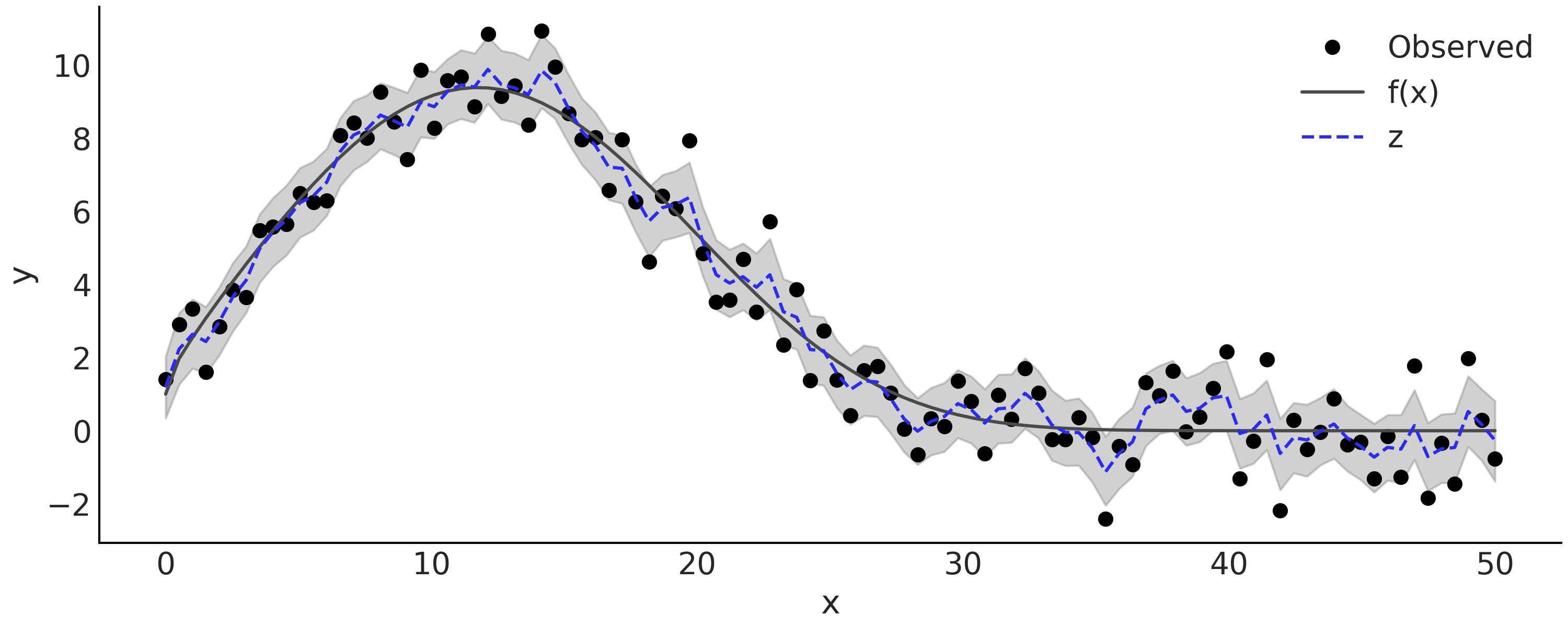
Fig. 113 来自 \(y \sim \text{Normal}(f(x), 1)\) 的模拟观测结果 \(f(x) = e^{1 + x^{0.5} - e^{\frac{x}{15} }}\)，以及推断的隐高斯随机游走。灰色半透明区域是隐高斯随机游走 \(z\) 的后验 \(94\%\) HDI 区间，后验均值图为蓝色虚线。

自回归过程还有一些其他有趣的性质，与高斯过程 [52] 有关。例如，你可能会发现单单靠自回归模型无法捕获长期的趋势。尽管模型对观测数据拟合得很好，但预测结果会快速回归到最后几个时间步的均值，与均值函数为常数的高斯过程表现相似 9 。

自回归分量作为一个加性的趋势性分量，可能会给模型推断带来一些挑战。例如，难以适应大规模数据，因为我们需要添加一个与时间观测序列大小相同的随机变量。当趋势性分量和自回归过程都灵活时，我们可能会得到一个无法辨识的模型，因为自回归过程本身已经有能力近似观测数据的潜在趋势（平滑函数）了。

6.3.3 移动平均自回归 (S)AR(I)MA(X)

许多经典的时间序列模型，共享一个相似的类自回归模式，其中在时间 \(t\) 处存在一些依赖于当前观测值（和/或 \(t-k\) 处的另外一个参数值）的隐参数。其中两个典型的例子是：

• 自回归条件异方差 ( ARCH ) 模型 ，该模型中残差的尺度会随时间变化；

• 移动平均 ( MA ) 模型，该模型在时间序列的均值上，加入历史时间步残差的某种线性组合值作为当前时间步的残差。

这些经典的时间序列模型，可以组合形成更复杂的模型。其中一种扩展是 具有外生回归量的整合移动平均季节性自回归模型（ Seasonal AutoRegressive Integrated Moving Average with eXogenous regressors model, SARIMAX）。虽然命名看起来吓人，但基本上就是自回归和移动平均模型的直接组合。用移动平均来扩展自回归模型，可以得到具有一般性的 自回归移动平均（ ARMA ） 模型：

(53)\[\begin{split}\begin{split} y_t & = \alpha + \sum_{i=1}^{p}\phi_i y_{t-i} + \sum_{j=1}^{q}\theta_j \epsilon_{t-j} + \epsilon_t \\ \epsilon_t & \sim \mathcal{N}(0, \sigma^2) \end{split}\end{split}\]

其中 \(p\) 是自回归模型的阶数，\(q\) 是移动平均模型的阶数。通常会将此模型记为 \(ARMA(p, q)\) 。进一步的，对于移动平均季节性自回归模型（ SARMA ），我们有：

(54)\[\begin{split} y_t = \alpha + \sum_{i=1}^{p}\phi_i y_{t-period-i} + \sum_{j=1}^{q}\theta_j \epsilon_{t-period-j} + \epsilon_t \end{split}\]

而在 整合移动平均自回归模型（AutoRegressive Integrated Moving Average, ARIMA） 中，”整合“是指对原始观测值进行差分处理，以使生成一个平稳的时间序列（即用当前时间步与之前时间步的数据值之差来代替当前数据值）。原始观测值被差分的次数被称为 整合阶数（ Order of Integration ） ，表示为 \(I(d)\) 。如果一个时间序列重复做 \(d\) 次差分后仍然能够生成平稳序列，就称其被整合到了 \(d\) 阶。遵从 Box et al. [57] 的定义 ，我们将时间观测序列的差分作为预处理步骤，来解释 \(ARIMA(p,d,q)\) 模型的 \(I(d)\) 部分，并将差分结果序列建模为一个带 \(ARMA(p,q)\) 的平稳过程。该运算本身在 Python 中相当普遍，可以使用 numpy.diff 实现，其中计算的第一个差分是沿给定轴的 delta_y[i] = y[i] - y[i-1]，通过在给定轴上递归重复相同运算来计算更高阶的差分结果数组。

如果我们有一个额外的回归量 \(\mathbf{X}\)，并将上述模型中的 \(\alpha\) 替换为线性预测 \(\mathbf{X} \beta\) 。如果模型设置 \(d > 0\)，则我们也会对 \(\mathbf{X}\) 做相应的差分处理。

此外请注意，我们可以有季节性回归（ SARIMA ）或外生回归（ ARIMAX ），但不能同时有。

(S)AR(I)MA(X) 的概念

整合移动平均自回归（ ARIMA ）模型通常表示为 \(ARIMA(p,d,q)\)，也就是说，我们有一个自回归阶数为 \(p\) 、整合度数为 \(d\) 、移动平均阶数为 \(q\) 的自回归模型。因此，\(ARIMA(1,0,0)\) 等价于 \(AR(1)\)。

季节性 ARIMA 模型通常被表示为 \(\text{SARIMA}(p,d,q)(P,D,Q)_{s}\)，其中 \(s\) 表示每个季节的周期数，而大写的 \(P\)、\(D\)、\(Q\) 则分别是模型 \(p\)、\(d\)、\(q\) 的季节性计数部分。有时季节性 ARIMA 也表示为 \(\text{SARIMA}(p,d,q)(P,D,Q,s)\)。

如果 ARIMA 模型 存在外生的回归量，则通常记为 \(\text{ARIMAX}(p,d,q)\mathbf{X}[k]\) ，其中 \(\mathbf{X}[k]\) 表示我们的设计矩阵 \(\mathbf{X}\) 包含 \(k\) 列。

作为本章的第二个例子，我们将使用不同的 ARIMA 模型 对美国从 \(1948\) 年到 \(1979\) 年的月活产率时间序列进行建模[58]。数据显示在 Fig. 114 中。

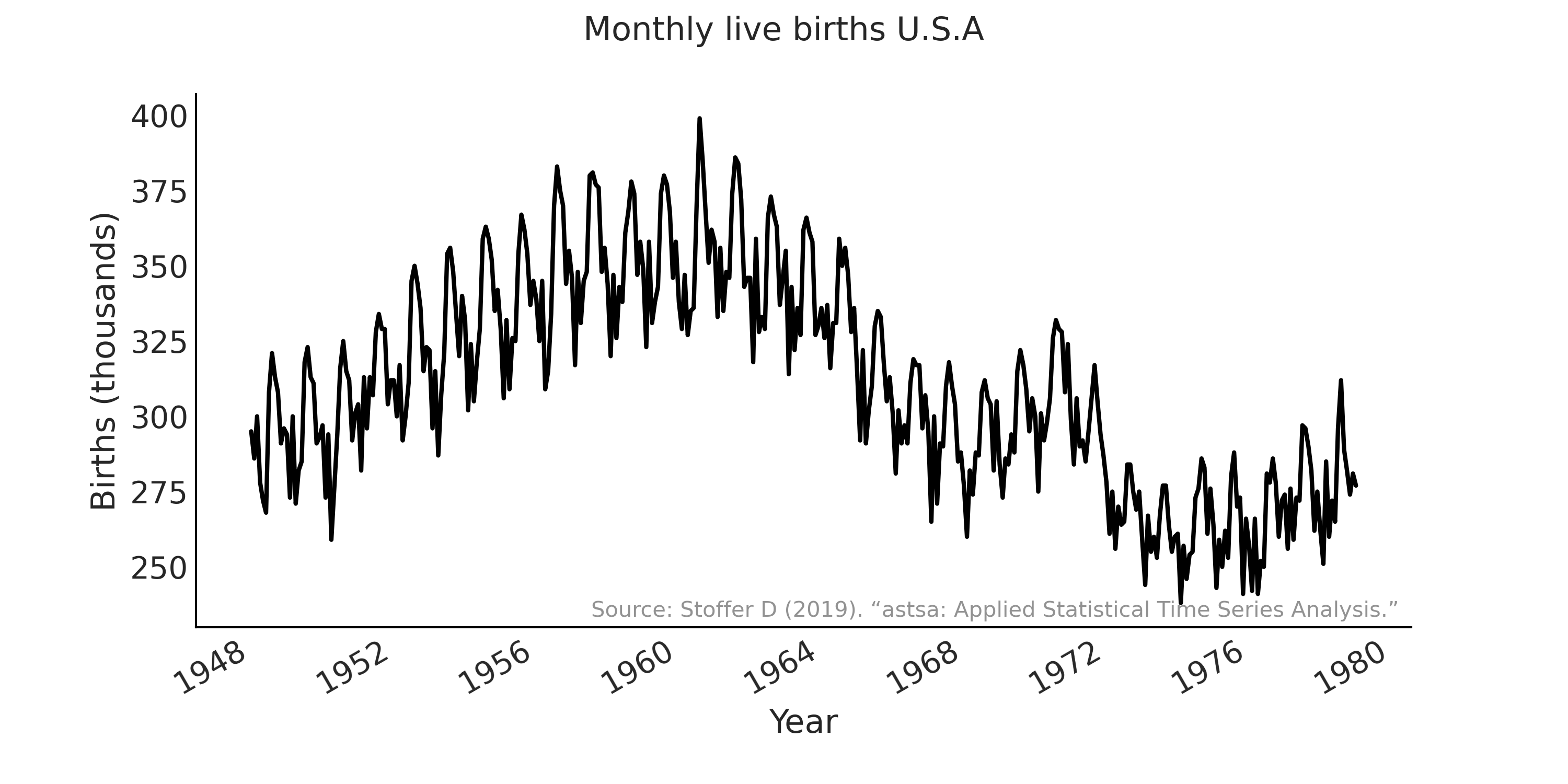
Fig. 114 美国的月活产婴儿（1948-1979 年）。 \(Y\) 轴显示出生人数（以千计）。

我们从 \(\text{SARIMA}(1, 1, 1)(1, 1, 1)_{12}\) 模型开始。首先，在代码 sarima_preprocess 中加载和预处理时间观测序列。

Listing 88 sarima_preprocess

us_monthly_birth = pd.read_csv("../data/monthly_birth_usa.csv")
us_monthly_birth["date_month"] = pd.to_datetime(us_monthly_birth["date_month"])
us_monthly_birth.set_index("date_month", drop=True, inplace=True)

# y ~ Sarima(1,1,1)(1,1,1)[12]
p, d, q = (1, 1, 1)
P, D, Q, period = (1, 1, 1, 12)
# Time series data: us_monthly_birth.shape = (372,)
observed = us_monthly_birth["birth_in_thousands"].values
# Integrated to seasonal order $D$
for _ in range(D):
    observed = observed[period:] - observed[:-period]
# Integrated to order $d$
observed = tf.constant(np.diff(observed, n=d), tf.float32)

在撰写本文时，TFP 没有专门的 ARMA 分布 。为了运行 SARIMA 模型的推断，TFP 需要一个 Python 的 callable 可调用对象来表示对数后验密度函数（ 最大值为某个常数 ） [30] 。在此情况下，可以将其实现为似然函数 \(\text{SARMA}(1, 1)(1, 1)_{12}\)（ 注： 整合部分 \(\text{I}\) 通过差分预处理实现 ）。

我们在代码 sarima_likelihood 使用 tf.while_loop 构造残差时间序列 \(\epsilon_t\) ，并在高斯分布上进行估计 10 。从编程角度来看，这里最大的挑战是当我们对时间序列进行索引时，确保张量形状是正确的。为了避免额外的控制流来检查索引是否有效（ 例如，当 \(t=0\) 时，我们是不能索引 \(t-1\) 和 \(t-period-1\) 的 ），采用零对时间序列进行了填充。

Listing 89 sarima_likelihood

def likelihood(mu0, sigma, phi, theta, sphi, stheta):
    batch_shape = tf.shape(mu0)
    y_extended = tf.concat(
        [tf.zeros(tf.concat([[r], batch_shape], axis=0), dtype=mu0.dtype),
        tf.einsum("...,j->j...",
                  tf.ones_like(mu0, dtype=observed.dtype),
                  observed)],
        axis=0)
    eps_t = tf.zeros_like(y_extended, dtype=observed.dtype)

    def arma_onestep(t, eps_t):
        t_shift = t + r
        # AR
        y_past = tf.gather(y_extended, t_shift - (np.arange(p) + 1))
        ar = tf.einsum("...p,p...->...", phi, y_past)
        # MA
        eps_past = tf.gather(eps_t, t_shift - (np.arange(q) + 1))
        ma = tf.einsum("...q,q...->...", theta, eps_past)
        # Seasonal AR
        sy_past = tf.gather(y_extended, t_shift - (np.arange(P) + 1) * period)
        sar = tf.einsum("...p,p...->...", sphi, sy_past)
        # Seasonal MA
        seps_past = tf.gather(eps_t, t_shift - (np.arange(Q) + 1) * period)
        sma = tf.einsum("...q,q...->...", stheta, seps_past)

        mu_at_t = ar + ma + sar + sma + mu0
        eps_update = tf.gather(y_extended, t_shift) - mu_at_t
        epsilon_t_next = tf.tensor_scatter_nd_update(
            eps_t, [[t_shift]], eps_update[None, ...])
        return t+1, epsilon_t_next

    t, eps_output_ = tf.while_loop(
        lambda t, *_: t < observed.shape[-1],
        arma_onestep,
        loop_vars=(0, eps_t),
        maximum_iterations=observed.shape[-1])
    eps_output = eps_output_[r:]
    return tf.reduce_sum(
        tfd.Normal(0, sigma[None, ...]).log_prob(eps_output), axis=0)

在代码 sarima_posterior 中，我们为未知参数（ mu0、sigma、phi、theta、sphi 和 stheta ）添加了先验，并创建了用于推断的后验密度函数 target_log_prob_fn 11 。

Listing 90 sarima_posterior

@tfd.JointDistributionCoroutine
def sarima_priors():
    mu0 = yield root(tfd.StudentT(df=6, loc=0, scale=2.5, name='mu0'))
    sigma = yield root(tfd.HalfStudentT(df=7, loc=0, scale=1., name='sigma'))

    phi = yield root(tfd.Sample(tfd.Normal(0, 0.5), p, name='phi'))
    theta = yield root(tfd.Sample(tfd.Normal(0, 0.5), q, name='theta'))
    sphi = yield root(tfd.Sample(tfd.Normal(0, 0.5), P, name='sphi'))
    stheta = yield root(tfd.Sample(tfd.Normal(0, 0.5), Q, name='stheta'))

target_log_prob_fn = lambda *x: sarima_priors.log_prob(*x) + likelihood(*x)

代码 sarima_preprocess 中时间序列的预处理可以解释 整合 部分，代码 sarima_likelihood 中实现的似然函数可以重构为一个可灵活生成不同 SARIMA 似然函数 的 Python 语言 helper 类。例如，Table 13 显示了代码 sarima_posterior 中的 $\(\text{SARIMA}(1,1,1)(1,1,1)_{12}\) 模型与相似的 \(\text{SARIMA}(0,1,2)(1,1,1)_{12}\) 模型之间的比较。

Table 13 使用 LOO（对数标度）对不同 SARIMA 模型进行模型比较的汇总数据。

	rank	loo	p_loo	d_loo	weight	se	dse
\(\text{SARIMA}(0,1,2)(1,1,1)_{12}\)	0	-1235.60	7.51	0.00	0.5	15.41	0.00
\(\text{SARIMA}(1,1,1)(1,1,1)_{12}\)	1	-1235.97	8.30	0.37	0.5	15.47	6.29

6.4 状态空间模型

在代码 sarima_likelihood 所指定模型的对数似然函数中，我们对时间步进行迭代，以便以观测为条件创建一些隐变量。实际上，除非模型非常具体和简单以至于能够使用向量化操作（例如，每两个连续时间步长之间的马尔可夫依赖关系可以将生成过程简化为向量化操作，而非迭代），否则迭代模式是表达时间序列模型的一种非常自然的方式。

状态空间模型（ Status Space Model ） 是这种迭代模式的一种通用形式，该模型对一个离散时间过程进行建模，假设在每个时间步，存在一些由前一步 \(X_{t-1}\) 演变而来隐状态 \(X_t\) （ 马尔可夫序列 ），而观测值 \(Y_t\) 则是从 \(X_t\) 所在的隐状态空间到观测空间的某种投影 12 ：

(55)\[\begin{split}\begin{split} X_0 & \sim p(X_0) \\ \text{for t in 0...T:} \\ Y_t & \sim p^{\psi}(Y_t \mid X_t) \\ X_{t+1} & \sim p^{\theta}(X_{t+1} \mid X_{t}) \end{split}\end{split}\]

其中 \(p(X_0)\) 是时间步 \(0\) 处隐状态的先验分布，\(p^{\theta}(X_{t+1} \mid X_t)\) 是由参数向量 \(\theta\) 参数化的转移概率， 其中 \(\theta\) 描述了某种系统动力学。\(p^{\psi}(Y_t \mid X_t)\) 是由向量 \(\psi\) 参数化的观测概率，描述了时间 \(t\) 时隐状态条件下的测量值。

实现高效计算的状态空间模型

使用 tf.while_loop 或 tf.scan 等 API 实现的状态空间模型和数学公式之间存在某种调谐。与使用 Python 的 for 循环或 while 循环不同，在 TFP 中，需要将循环体编译成一个函数，该函数采用相同的张量结构作为输入和输出。这种函数风格的实现方式有助于显式地表示 “在每个时间步隐状态是如何转换的？” 以及 “隐状态如果转换到为观测结果的？”。值得注意的是，实现状态空间模型及其相关推断算法（ 如卡尔曼滤波器 ）也涉及在何处放置初始计算的设计决策。在上式中，我们在初始隐条件上放置了一个先验，并且第一个观测值直接来自初始状态的测量值。不过，在第 \(0\) 步中，对隐状态进行转换同样有效，然后通过修改先验分布进行第一次观测，这两种方法是等效的。

然而，在为时间序列问题实现滤波时，在张量的形状处理上有一些微妙的技巧。主要挑战是时间维的放置位置。一个明显选择是将其放置在轴 \(0\) 上，因为使用 t 作为时间索引来执行 time_series[t] 是很自然的事情。使用 tf.scan 或 theano.scan 等循环结构在时间序列上实现循环时，会自动将时间维度放在轴 \(0\) 上。但这与通常作为引导轴的批处理维有冲突。例如，如果我们想对 \(N\) 批的 \(k\) 维时间序列向量化，每个时间序列总共有 \(T\) 个时间戳，则数组的形状为 [N, T, ...]，但 tf.scan 的输出形状为 [T, N, ...] 。目前，建模人员似乎不可避免地需要对 scan 的输出执行转置，以使其与输入张量的批处理维和时间维语义相匹配。

有了时间序列问题的状态空间表示，我们就处在了一个序列分析的框架中。该框架通常包括滤波、平滑等任务：

• 滤波：以时间步 \(k\) 之前的观测作为条件，计算隐状态 \(X_k\) 的边缘分布 \(p(X_k \mid y_{0:k}), k = 0,...,T\) ； 然后将上述滤波扩展到未来 \(n\) 步，即做出预测 \(p(X_k+n \mid y_{0:k}), k = 0,... ,T, n=1, 2,...\)

• 平滑：类似于滤波，但会尝试以所有观测为条件计算隐状态 \(X_k\) 的边缘分布：\(p(X_k \mid y_{0:T}), k = 0 ,...,T\) 。

注意：滤波和平滑中的下标 \(y_{0:\dots}\) 有所不同，滤波以 \(y_{0:k}\) 为条件，而平滑以 \(y_{0:T}\) 为条件。

事实上，从滤波和平滑的视角来建模时间序列有着悠久的历史。例如，我们计算 ARMA 模型的对数似然时，采取的方式就可以看作是一个滤波问题，其中观测数据被解构为一些隐含的不可观测状态。

6.4.1 线性高斯状态空间模型与卡尔曼滤波

线性高斯状态空间模型也许是最著名的状态空间模型。在该模型中，假设存在隐状态 \(X_t\) ，观测 \(Y_t\) 呈（多元）高斯分布，并且状态转移函数和观测函数都是线性的：

(56)\[\begin{split}\begin{split} Y_t & = \mathbf{H}_t X_t + \epsilon_t \\ X_t & = \mathbf{F}_t X_{t-1} + \eta_t \end{split}\end{split}\]

其中 \(\epsilon_t \sim \mathcal{N}(0, \mathbf{R}_t)\) 和 \(\eta_t \sim \mathcal{N}(0, \mathbf{Q}_t)\) 是噪声分量。

变量 (\(\mathbf{H}_t\), \(\mathbf{F}_t\)) 是描述线性变换的矩阵。通常 \(\mathbf{F}_t\) 是方阵，代表相邻时间步之间的线性状态转移函数；\(\mathbf{H} _t\) 的秩低于 \(\mathbf{F}_t\)，表示隐状态到观测之间的线性观测函数； \(\mathbf{R}_t\), \(\mathbf{Q}_t\) 是协方差矩阵（正半定矩阵）。你还可以在 11.1.11 马尔可夫链 中找到一些比较直观的示例。

由于 \(\epsilon_t\) 和 \(\eta_t\) 都是服从高斯分布的随机变量，而上述线性函数只是对高斯随机变量做了仿射变换，因此导致 \(X_t\) 和 \(Y_t\) 也服从高斯分布。也就是说，先验（ \(t-1\) 时的状态 ）和后验（ \(t\) 时的状态 ）之间存在共轭性质，这使获得贝叶斯滤波公式的解析解成为可能，即卡尔曼滤波器（Kalman，1960）。作为共轭贝叶斯模型最重要的应用之一，卡尔曼滤波器帮助人类登陆月球，并且至今在许多领域仍然被广泛使用。

为了直观地理解卡尔曼滤波器，首先看一下线性高斯状态空间模型从时间 \(t-1\) 到 \(t\) 的生成过程：

(57)\[\begin{split}\begin{split} X_t \sim p(X_t \mid X_{t-1}) & \equiv \mathcal{N}(\mathbf{F}_{t} X_{t-1}, \mathbf{Q}_{t}) \\ Y_t \sim p(Y_t \mid X_t) & \equiv \mathcal{N}(\mathbf{H}_t X_t, \mathbf{R}_t) \end{split}\end{split}\]

其中 \(X_t\) 和 \(Y_t\) 的条件概率分布表示为 \(p(.)\)（ 此处使用 \(\equiv\) 表示该条件分布为多元高斯分布 ）。请注意，\(X_t\) 仅取决于上一个时间步的状态 \(X_{t-1}\) ，而不取决于之前的历史观测。这意味着，生成过程可以首先生成一个隐时间序列 \(X_t,\ t = 0...T\) ， 然后再将整个隐时间序列投射到观测空间中。在贝叶斯滤波场景中，\(Y_t\) 是可观测的，因此被用于对隐状态 \(X_t\) 进行更新，类似于在静态模型中用（观测数据的）似然去更新先验：

(58)\[\begin{split}\begin{split} X_0 \sim p(X_0 \mid m_0, \mathbf{P}_0) & \equiv \mathcal{N}(m_0, \mathbf{P}_0) \\ X_{t \mid t-1} \sim p(X_{t \mid t-1} \mid Y_{0:t-1}) & \equiv \mathcal{N}(m_{t \mid t-1}, \mathbf{P}_{t \mid t-1}) \\ X_{t \mid t} \sim p(X_{t \mid t} \mid Y_{0:t}) & \equiv \mathcal{N}(m_{t \mid t}, \mathbf{P}_{t \mid t}) \\ Y_t \sim p(Y_t \mid Y_{0:t-1}) & \equiv \mathcal{N}(\mathbf{H}_t m_{t \mid t-1}, \mathbf{S}_t) \end{split}\end{split}\]

其中 \(m_t\) 和 \(\mathbf{P}_t\) 表示隐状态 \(X_t\) 的均值和协方差矩阵。 \(X_{t \mid t-1}\) 是参数 \(m_{t \mid t-1}\) （预测均值）和 \(\mathbf{P}_{t \mid t-1}\) （预测协方差）下隐状态的预测值，而 \(X_{t \mid t}\) 是参数 \(m_{t \mid t}\) 和 \(\mathbf{P}_{t \mid t}\)下隐状态的滤波后结果。

公式 (58) 中的下标容易让人感到困惑，因此需要有一个高层视图来理解它：从上一个时间步开始，我们有一个滤波后状态 \(X_{t-1 \mid t-1} \) ；在应用转移矩阵 \(\mathbf{F}_{t}\) 后，得到一个预测的隐状态 \(X_{t \mid t-1}\) ；结合当前时间步的观测值，我们得到一个当前时间步的滤波后新状态 \(X_{t \mid t}\) 。

公式 (58) 中，上述分布的参数是利用卡尔曼滤波的预测和更新步骤计算的：

• 预测步骤：

  (59)\[\begin{split}\begin{split} m_{t \mid t-1} & = \mathbf{F}_{t} m_{t-1 \mid t-1} \\ \mathbf{P}_{t \mid t-1} & = \mathbf{F}_{t} \mathbf{P}_{t-1 \mid t-1} \mathbf{F}_{t}^T + \mathbf{Q}_{t} \end{split}\end{split}\]

• 更新步骤

  (60)\[\begin{split}\begin{split} z_t & = Y_t - \mathbf{H}_t m_{t \mid t-1} \\ \mathbf{S}_t & = \mathbf{H}_t \mathbf{P}_{t \mid t-1} \mathbf{H}_t^T + \mathbf{R}_t \\ \mathbf{K}_t & = \mathbf{P}_{t \mid t-1} \mathbf{H}_t^T \mathbf{S}_t^{-1} \\ m_{t \mid t} & = m_{t \mid t-1} + \mathbf{K}_t z_t \\ \mathbf{P}_{t \mid t} & = \mathbf{P}_{t \mid t-1} - \mathbf{K}_t \mathbf{S}_t \mathbf{K}_t^T \end{split}\end{split}\]

卡尔曼滤波方程的推导主要使用了多元高斯联合分布。在实践中，还有一些技巧来确保计算在数值上是稳定的。例如，为了避免求矩阵 \(\mathbf{S}_t\) 的逆，在计算 \(\mathbf{P}_{t\mid t}\) 时使用 Jordan 范数 做更新，以确保结果为正定矩阵 [59]。在 TFP 中，线性高斯状态空间模型和卡尔曼滤波器可以通过分布tfd.LinearGaussianStateSpaceModel 很方便地实现。

在使用线性高斯状态空间模型做时间序列建模时，实践性的挑战之一是如何将未知参数表示为高斯隐状态。我们用一个简单的线性增长时间序列作为第一个示例进行演示（ 参见《贝叶斯滤波和平滑》 [60] 的第 \(3\) 章 ）：

Listing 91 linear_growth_model

theta0, theta1 = 1.2, 2.6
sigma = 0.4
num_timesteps = 100

time_stamp = tf.linspace(0., 1., num_timesteps)[..., None]
yhat = theta0 + theta1 * time_stamp
y = tfd.Normal(yhat, sigma).sample()

你可能会将代码 linear_growth_model 识别为简单线性回归。要将其作为使用卡尔曼滤波器的滤波问题来处理，需要假设观测噪声 \(\sigma\) 已知，未知参数 \(\theta_0\) 和 \(\theta_1\) 服从高斯先验分布。

在状态空间形式中，有隐状态：

(61)\[\begin{split}X_t = \left[\begin{array}{ccc} \theta_0 \\ \theta_1 \\ \end{array}\right]\end{split}\]

由于隐状态不随时间变化，转移矩阵 \(F_t\) 是一个没有转移噪声的单位矩阵。观测矩阵描述了从隐空间到观测空间的转换，它是线性函数的矩阵形式 13 ：

(62)\[\begin{split}y_t = \theta_0 + \theta_1 * t = \left[\begin{array}{ccc} 1, t \\ \end{array}\right]\left[\begin{array}{ccc} \theta_0 \\ \theta_1 \\ \end{array}\right]\end{split}\]

用 tfd.LinearGaussianStateSpaceModel API 表示时，有：

Listing 92 tfd_lgssm_linear_growth

# X_0
initial_state_prior = tfd.MultivariateNormalDiag(
    loc=[0., 0.], scale_diag=[5., 5.])
# F_t
transition_matrix = lambda _: tf.linalg.LinearOperatorIdentity(2)
# eta_t ~ Normal(0, Q_t)
transition_noise = lambda _: tfd.MultivariateNormalDiag(
    loc=[0., 0.], scale_diag=[0., 0.])
# H_t
H = tf.concat([tf.ones_like(time_stamp), time_stamp], axis=-1)
observation_matrix = lambda t: tf.linalg.LinearOperatorFullMatrix(
    [tf.gather(H, t)])
# epsilon_t ~ Normal(0, R_t)
observation_noise = lambda _: tfd.MultivariateNormalDiag(
    loc=[0.], scale_diag=[sigma])

linear_growth_model = tfd.LinearGaussianStateSpaceModel(
    num_timesteps=num_timesteps,
    transition_matrix=transition_matrix,
    transition_noise=transition_noise,
    observation_matrix=observation_matrix,
    observation_noise=observation_noise,
    initial_state_prior=initial_state_prior)

我们可以应用卡尔曼滤波器获得 \(\theta_0\) 和 \(\theta_1\) 的后验分布：

Listing 93 tfd_lgssm_linear_growth_filter

# Run the Kalman filter
(
    log_likelihoods,
    mt_filtered, Pt_filtered,
    mt_predicted, Pt_predicted,
    observation_means, observation_cov  # observation_cov is S_t
) = linear_growth_model.forward_filter(y)

可以在 Fig. 115 中将卡尔曼滤波器的结果（即迭代地观测每个时间步）与解析结果（即观测完整的时间序列）进行比较。

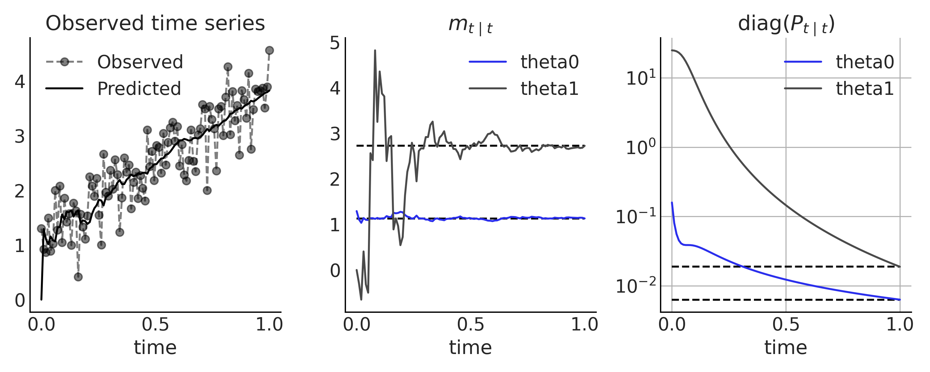
Fig. 115 线性增长时间序列模型，使用卡尔曼滤波器进行推断。在第一个子图中，展示了观测数据（用虚线连接的灰点）和来自卡尔曼滤波器的单步预测（ 黑色实线中的 \(H_t m_{t \mid t-1}\) ）。将观测每个时间步之后获得的隐状态 \(X_t\) 的后验分布，与中间子图和右侧子图中使用所有数据获得的解析解（黑色实线）进行比较。

6.4.2 ARIMA 模型的状态空间表示

状态空间模型是一种概括了许多经典时间序列模型的统一方法。但如何以状态空间形式表达传统模型可能并不总是很明显。在本节中，我们将了解如何表达更复杂的线性高斯状态空间模型：ARMA 和 ARIMA。

回想前面的 \(ARMA(p,q)\) 模型的公式 (53)，我们有自回归系数 \(\phi_i\)、移动平均系数 \(\theta_j\) 和噪声参数 \(\sigma\) 。使用 \(\sigma\) 来对观测噪声的分布 \(R_t\) 进行参数化，很具有吸引力。然而，在公式 (53) 中，利用先前时间步的噪声所做的移动平均，需要我们存储当前噪声。唯一的解决办法是将其形式化为转移噪声，使其成为隐状态 \(X_t\) 的一部分。

可以将公式 (53) 重新表述为：

(63)\[y_t = \sum_{i=1}^{r}\phi_i y_{t-i} + \sum_{i=1}^{r-1}\theta_i \epsilon_{t-i} + \epsilon_t\]

公式 (53) 中的常数项 \(\alpha\) 被略去，并且常数项 \(r = \max(p, q+1)\) 。我们在需要时用零来填充参数 \(\phi\) 和 \(\theta\) ，以便其长度均为 \(r\) 。因此状态方程中的 \(X_t\) 分量为：

(64)\[\begin{split}\mathbf{F}_t = \mathbf{F} = \left[\begin{array}{cccc} \phi_1 & 1 & \cdots & 0 \\ \vdots & \vdots & \ddots & \vdots \\ \phi_{r-1} & 0 & \cdots & 1 \\ \phi_r & 0 & \cdots & 0 \end{array}\right], \\ \mathbf{A} = \left[\begin{array}{c} 1\\ \theta_1 \\ \vdots \\ \theta_{r-1} \\ \end{array}\right], \eta'_{t+1} \sim \mathcal{N}(0, \sigma^2), \eta_t = \mathbf{A} \eta'_{t+1}\end{split}\]

隐状态为：

(65)\[\begin{split}X_t = \left[\begin{array}{ccc} y_t \\ \phi_2 y_{t-1} + \dots + \phi_r y_{t-r+1} + \theta_1 \eta'_t + \dots + \theta_{r-1} \eta'_{t-r+2} \\ \phi_3 y_{t-1} + \dots + \phi_r y_{t-r+2} + \theta_2 \eta'_t + \dots + \theta_{r-1} \eta'_{t-r+3} \\ \vdots \\ \phi_r y_{t-1} + \theta_{r-1} \eta'_t \end{array}\right]\end{split}\]

观测矩阵只是一个索引矩阵 \(\mathbf{H}_t = [1, 0, 0, \dots, 0]\)，观测方程为 \(y_t = \mathbf{H}_t X_t\) 14 。

例如，\(ARMA(2,1)\) 模型的状态空间表示为：

(66)\[\begin{split}\begin{split} \left[\begin{array}{ccc} y_{t+1}\\ \phi_2 y_t + \theta_1 \eta'_{t+1}\\ \end{array}\right] & = \left[\begin{array}{ccc} \phi_1 & 1\\ \phi_2 & 0\\ \end{array}\right] \left[\begin{array}{ccc} y_t\\ \phi_2 y_{t-1} + \theta_1 \eta'_t\\ \end{array}\right] + \left[\begin{array}{ccc} 1\\ \theta_1\\ \end{array}\right] \eta'_{t+1}\\ \eta'_{t+1} & \sim \mathcal{N}(0, \sigma^2) \end{split}\end{split}\]

你可能注意到状态转移函数与前面的定义略有不同，因为转换噪声不是从多元高斯分布中抽取的。 \(\eta\) 的协方差矩阵是 \(\mathbf{Q}_t = \mathbf{A} \sigma^2 \mathbf{A}^T\) ，在当前情况下，会产生奇异的随机变量 \(\eta\) 。但无论如何，我们现在可以在 TFP 中定义模型了。例如，在代码 tfd_lgssm_arma_simulate 中，我们定义了一个 \(ARMA(2,1)\) 模型，其中 \(\phi = [-0.1, 0.5]\) 、 \(\theta = -0.25\) 、 \(\sigma = 1.25\) ，并抽取了一个随机时间序列。

Listing 94 tfd_lgssm_arma_simulate

num_timesteps = 300
phi1 = -.1
phi2 = .5
theta1 = -.25
sigma = 1.25

# X_0
initial_state_prior = tfd.MultivariateNormalDiag(
   scale_diag=[sigma, sigma])
# F_t
transition_matrix = lambda _: tf.linalg.LinearOperatorFullMatrix(
   [[phi1, 1], [phi2, 0]])
# eta_t ~ Normal(0, Q_t)
R_t = tf.constant([[sigma], [sigma*theta1]])
Q_t_tril = tf.concat([R_t, tf.zeros_like(R_t)], axis=-1)
transition_noise = lambda _: tfd.MultivariateNormalTriL(
   scale_tril=Q_t_tril)
# H_t
observation_matrix = lambda t: tf.linalg.LinearOperatorFullMatrix(
   [[1., 0.]])
# epsilon_t ~ Normal(0, 0)
observation_noise = lambda _: tfd.MultivariateNormalDiag(
   loc=[0.], scale_diag=[0.])

arma = tfd.LinearGaussianStateSpaceModel(
   num_timesteps=num_timesteps,
   transition_matrix=transition_matrix,
   transition_noise=transition_noise,
   observation_matrix=observation_matrix,
   observation_noise=observation_noise,
   initial_state_prior=initial_state_prior
   )

sim_ts = arma.sample()  # Simulate from the model

添加适当先验并做一些重写可以更好地处理张量的形状，我们在代码 tfd_lgssm_arma_with_prior 中得到了一个完整的生成式 \(ARMA(2,1)\) 模型。

由于使用了 tfd.JointDistributionCoroutine 模型，因此对（模拟的）数据 sim_ts 和推断进行调整比较简单。请注意，未知参数并非隐状态 \(X_t\) 的一部分，因此不能像卡尔曼滤波那样做贝叶斯滤波推导，而是使用标准的 MCMC 方法进行推断。 Fig. 116 中展示了其后验样本的轨迹图。

Listing 95 tfd_lgssm_arma_with_prior

@tfd.JointDistributionCoroutine
def arma_lgssm():
    sigma = yield root(tfd.HalfStudentT(df=7, loc=0, scale=1., name="sigma"))
    phi = yield root(tfd.Sample(tfd.Normal(0, 0.5), 2, name="phi"))
    theta = yield root(tfd.Sample(tfd.Normal(0, 0.5), 1, name="theta"))
    # Prior for initial state
    init_scale_diag = tf.concat([sigma[..., None], sigma[..., None]], axis=-1)
    initial_state_prior = tfd.MultivariateNormalDiag(
        scale_diag=init_scale_diag)
    
    F_t = tf.concat([phi[..., None],
                     tf.concat([tf.ones_like(phi[..., 0, None]),
                                tf.zeros_like(phi[..., 0, None])],
                               axis=-1)[..., None]],
                    axis=-1)
    transition_matrix = lambda _: tf.linalg.LinearOperatorFullMatrix(F_t)
    
    transition_scale_tril = tf.concat(
        [sigma[..., None], theta * sigma[..., None]], axis=-1)[..., None]
    scale_tril = tf.concat(
        [transition_scale_tril,
         tf.zeros_like(transition_scale_tril)],
        axis=-1)
    transition_noise = lambda _: tfd.MultivariateNormalTriL(
        scale_tril=scale_tril)
    
    observation_matrix = lambda t: tf.linalg.LinearOperatorFullMatrix([[1., 0.]])
    observation_noise = lambda t: tfd.MultivariateNormalDiag(
        loc=[0], scale_diag=[0.])

    arma = yield tfd.LinearGaussianStateSpaceModel(
            num_timesteps=num_timesteps,
            transition_matrix=transition_matrix,
            transition_noise=transition_noise,
            observation_matrix=observation_matrix,
            observation_noise=observation_noise,
            initial_state_prior=initial_state_prior,
            name="arma")

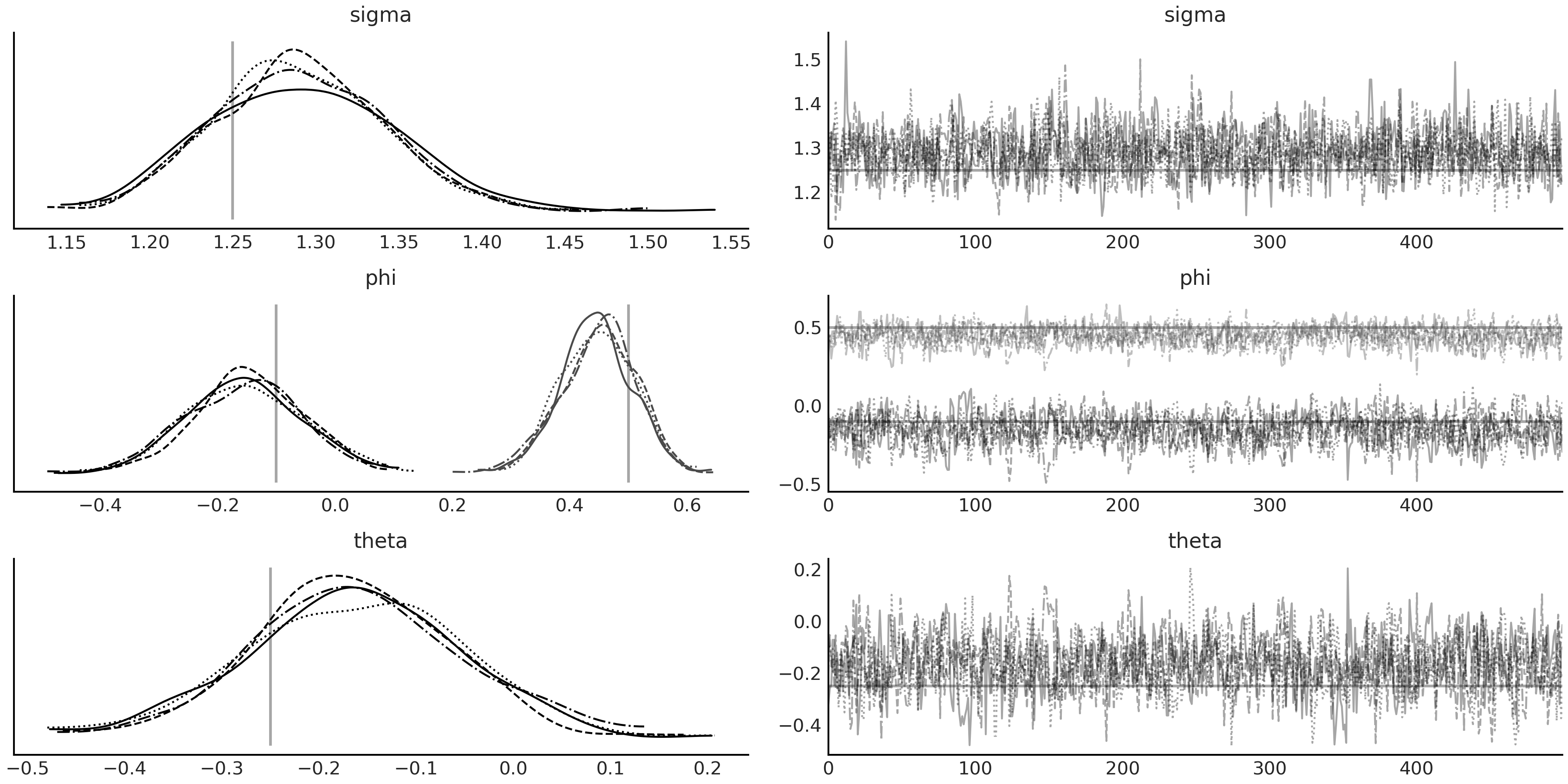
Fig. 116 代码 tfd_lgssm_arma_with_prior 中的 \(ARMA(2,1)\) 模型 arma_lgssm 的 MCMC 采样结果，以代码 tfd_lgssm_arma_simulate 中生成的模拟数据 sim_ts 为条件。参数的真实值在后验密度图中绘制为垂线，在轨迹图中绘制为水平线。

结合在预处理阶段对观测时间序列的差分处理，我们可以进一步将该形式用于 \(d>0\) 的 ARIMA 建模。状态空间模型的表达形式提供了一个很重要的优势：我们可以更直接、更直观地写下生成过程，而无需在数据预处理步骤中的重复 \(d\) 次差分。

例如，考虑用 \(d=1\) 扩展上面的 \(ARMA(2,1)\) 模型，有 \(\Delta y_t = y_t - y_{t-1}\)，这意味着 \(y_t = y_{t-1} + \Delta y_t\)，我们可以将观测矩阵定义为 \(\mathbf{H}_t = [1, 1, 0]\) ，其中隐状态 \(X_t\) 和状态转移矩阵为：

(67)\[\begin{split}\begin{split} \left[\begin{array}{ccc} y_{t-1} + \Delta y_t \\ \phi_1 \Delta y_t + \phi_2 \Delta y_{t-1} + \eta'_{t+1} + \theta_1 \eta'_t\\ \phi_2 \Delta y_t + \theta_1 \eta'_{t+1}\\ \end{array}\right] & = \left[\begin{array}{ccc} 1 & 1 & 0 \\ 0 & \phi_1 & 1\\ 0 & \phi_2 & 0\\ \end{array}\right] \left[\begin{array}{ccc} y_{t-1}\\ \Delta y_t \\ \phi_2 \Delta y_{t-1} + \theta_1 \eta'_t\\ \end{array}\right] + \left[\begin{array}{ccc} 0 \\ 1 \\ \theta_1\\ \end{array}\right] \eta'_{t+1} \end{split}\end{split}\]

如你所见，虽然参数化导致了更大的隐状态向量 \(X_t\)，但参数数量保持不变。此外，该模型在 \(y_t\) 而不是 \(\Delta y_t\) 中是生成式的。上述方法在指定初始状态 \(X_0\) 的分布时可能存在挑战，因为第一个元素 ( \(y_0\) ) 现在是非平稳的。在实践中，可以在中心化处理之后，围绕时间序列的初始值分配一个信息性先验。你可以在 Durbin and Koopman [61] 中找到有关此主题的更多讨论，以及对状态空间模型的深入介绍。

6.4.3 贝叶斯结构化的时间序列

时间序列模型的线性高斯状态空间表达形式具有另一个优点，即它很容易与其他线性高斯状态空间模型一起扩展。为了将两个模型组合在一起，可以对隐空间中的两个高斯随机变量做连接。我们使用两个协方差矩阵生成一个块对角矩阵，连接事件轴上的均值。在观测空间中，该操作相当于对两个高斯随机变量求和。

更具体地说，有：

(68)\[\begin{split}\begin{split} \mathbf{F}_t & = \left[\begin{array}{ccc} \mathbf{F}_{\mathbf{1}, t} & 0 \\ 0 & \mathbf{F}_{\mathbf{2}, t}\\ \end{array}\right], \mathbf{Q}_t = \left[\begin{array}{ccc} \mathbf{Q}_{\mathbf{1}, t} & 0 \\ 0 & \mathbf{Q}_{\mathbf{2}, t}\\ \end{array}\right], X_t = \left[\begin{array}{ccc} X_{1,t} \\ X_{2,t}\\ \end{array}\right] \\ \mathbf{H}_t & = \left[\begin{array}{ccc} \mathbf{H}_{\mathbf{1}, t} & \mathbf{H}_{\mathbf{2}, t} \\ \end{array}\right], \mathbf{R}_t = \mathbf{R}_{\mathbf{1}, t} + \mathbf{R}_{\mathbf{2}, t}\\ \end{split}\end{split}\]

如果有一个不是线性高斯的时间序列模型 \(\mathcal{M}\) ，我们也可以将其合并到状态空间模型中。

为此，可以将每个时间步中来自模型 \(\mathcal{M}\) 的预测 \(\hat{\psi}_t\) 视为静态的已知值，并将其添加到观测噪声分布 \(\epsilon_t \sim N( \hat{\mu}_t + \hat{\psi}_t, R_t)\) 中。从概念上讲，我们可以将其理解为从 \(Y_t\) 中减去模型 \(\mathcal{M}\) 的预测，然后对结果进行建模，因此卡尔曼滤波器和其他线性高斯状态空间模型属性仍然成立。

这种 可组合性 的能力，使我们能够轻松地由多个小型线性高斯状态空间模型分量来构建更复杂的时间序列模型。我们可以分别为趋势性分量、季节性分量和误差项分别提供状态空间表示，并将其组合成通常所说的结构化时间序列模型或动态线性模型。 TFP 的 tfp.sts 模块提供了一种非常方便的方法来构建贝叶斯结构化时间序列，同时它还提供了用于解构分量、预测、推断和各种诊断的辅助函数。

例如，可以使用具有局部线性趋势性分量和季节性分量的结构化时间序列对每月出生数据进行建模，以解释代码 tfp_sts_example2 中的月模式。

Listing 96 tfp_sts_example2

def generate_bsts_model(observed=None):
    """
    Args:
        observed: Observed time series, tfp.sts use it to generate prior.
    """
    # Trend
    trend = tfp.sts.LocalLinearTrend(observed_time_series=observed)
    # Seasonal
    seasonal = tfp.sts.Seasonal(num_seasons=12, observed_time_series=observed)
    # Full model
    return tfp.sts.Sum([trend, seasonal], observed_time_series=observed)

observed = tf.constant(us_monthly_birth["birth_in_thousands"], dtype=tf.float32)
birth_model = generate_bsts_model(observed=observed)

# Generate the posterior distribution conditioned on the observed
target_log_prob_fn = birth_model.joint_log_prob(observed_time_series=observed)

我们可以检查 birth_model 中的每个分量：

Listing 97 tfp_sts_model

birth_model.components

[<tensorflow_probability.python.sts.local_linear_trend.LocalLinearTrend at ...>,
 <tensorflow_probability.python.sts.seasonal.Seasonal at ...>]

每个分量都由一些超参数参数化，这些超参数是我们想要进行推断的未知参数。它们不是隐状态 \(X_t\) 的组成部分，但有可能参数化生成 \(X_t\) 的先验。例如，我们可以检查季节性分量的参数：

Listing 98 tfp_sts_model_component

birth_model.components[1].parameters

[Parameter(name='drift_scale', prior=<tfp.distributions.LogNormal 
'Seasonal_LogNormal' batch_shape=[] event_shape=[] dtype=float32>,
bijector=<tensorflow_probability.python.bijectors.chain.Chain object at ...>)]

这里 STS 模型的季节性分量包含 \(12\) 个隐状态（每个月一个），但该分量仅包含 \(1\) 个参数（参数化隐状态的超参数）。你可能已经从上一节中的示例中注意到了未知参数的处理方式有所不同。在线性增长模型中，未知参数是隐状态 \(X_t\) 的组成部分，但在 ARIMA 模型中，未知参数参数化了 \(\mathbf{F}_t\) 和 \(\mathbf{Q}_t\)。对于后者，不能使用卡尔曼滤波器来推断这些参数。取而代之，隐状态被高效地边缘化了，不过我们仍然能够在推断完成后，通过运行以后验分布为条件的卡尔曼滤波器（表示为蒙特卡洛样本）来恢复它们。参数化的概念描述可以参见 Fig. 117 。

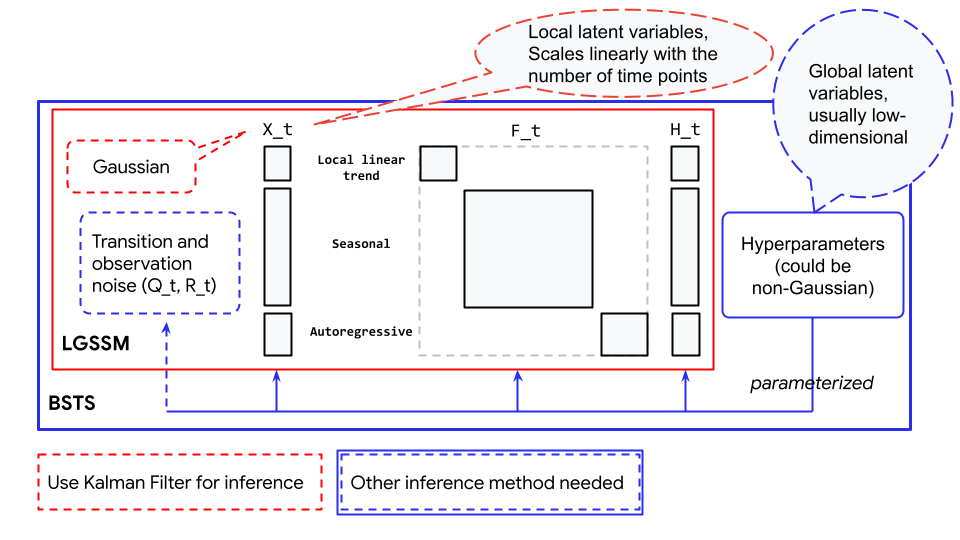
Fig. 117 贝叶斯结构化时间序列（蓝色框）与线性高斯状态空间模型（红色框）之间的关系。此处显示的线性高斯状态空间模型是一个包含局部线性趋势性分量、季节性分量和自回归分量的例子。

对结构化时间序列模型进行推断，在概念上可以理解为：从要推断的参数生成线性高斯状态空间模型、运行卡尔曼滤波器以获得数据似然、结合以参数当前值为条件的先验对数似然。不幸的是，遍历每个数据点的操作在计算上相当昂贵（尽管卡尔曼滤波器已经是一种非常有效的算法），因此在运行长时间序列时，拟合结构化时间序列可能无法很好地做相应大规模扩展。

在对结构化时间序列模型进行推断之后，我们可以使用来自 tfp.sts 的一些实用函数来预测和检查每个被推断的分量，见代码 tfp_sts_example2_result ，其结果显示在 Fig. 118 中。

Listing 99 tfp_sts_example2_result

# Using a subset of posterior samples.
parameter_samples = [x[-100:, 0, ...] for x in mcmc_samples]

# Get structual compoenent.
component_dists = tfp.sts.decompose_by_component(
    birth_model,
    observed_time_series=observed,
    parameter_samples=parameter_samples)

# Get forecast for n_steps.
n_steps = 36
forecast_dist = tfp.sts.forecast(
    birth_model,
    observed_time_series=observed,
    parameter_samples=parameter_samples,
    num_steps_forecast=n_steps)
birth_dates = us_monthly_birth.index
forecast_date = pd.date_range(
    start=birth_dates[-1] + np.timedelta64(1, "M"),
    end=birth_dates[-1] + np.timedelta64(1 + n_steps, "M"),
    freq="M")

fig, axes = plt.subplots(
    1 + len(component_dists.keys()), 1, figsize=(10, 9), sharex=True)

ax = axes[0]
ax.plot(us_monthly_birth, lw=1.5, label="observed")

forecast_mean = np.squeeze(forecast_dist.mean())
line = ax.plot(forecast_date, forecast_mean, lw=1.5,
               label="forecast mean", color="C4")

forecast_std = np.squeeze(forecast_dist.stddev())
ax.fill_between(forecast_date,
                forecast_mean - 2 * forecast_std,
                forecast_mean + 2 * forecast_std,
                color=line[0].get_color(), alpha=0.2)

for ax_, (key, dist) in zip(axes[1:], component_dists.items()):
    comp_mean, comp_std = np.squeeze(dist.mean()), np.squeeze(dist.stddev())
    line = ax_.plot(birth_dates, dist.mean(), lw=2.)
    ax_.fill_between(birth_dates,
                     comp_mean - 2 * comp_std,
                     comp_mean + 2 * comp_std,
                     alpha=0.2)
    ax_.set_title(key.name[:-1])

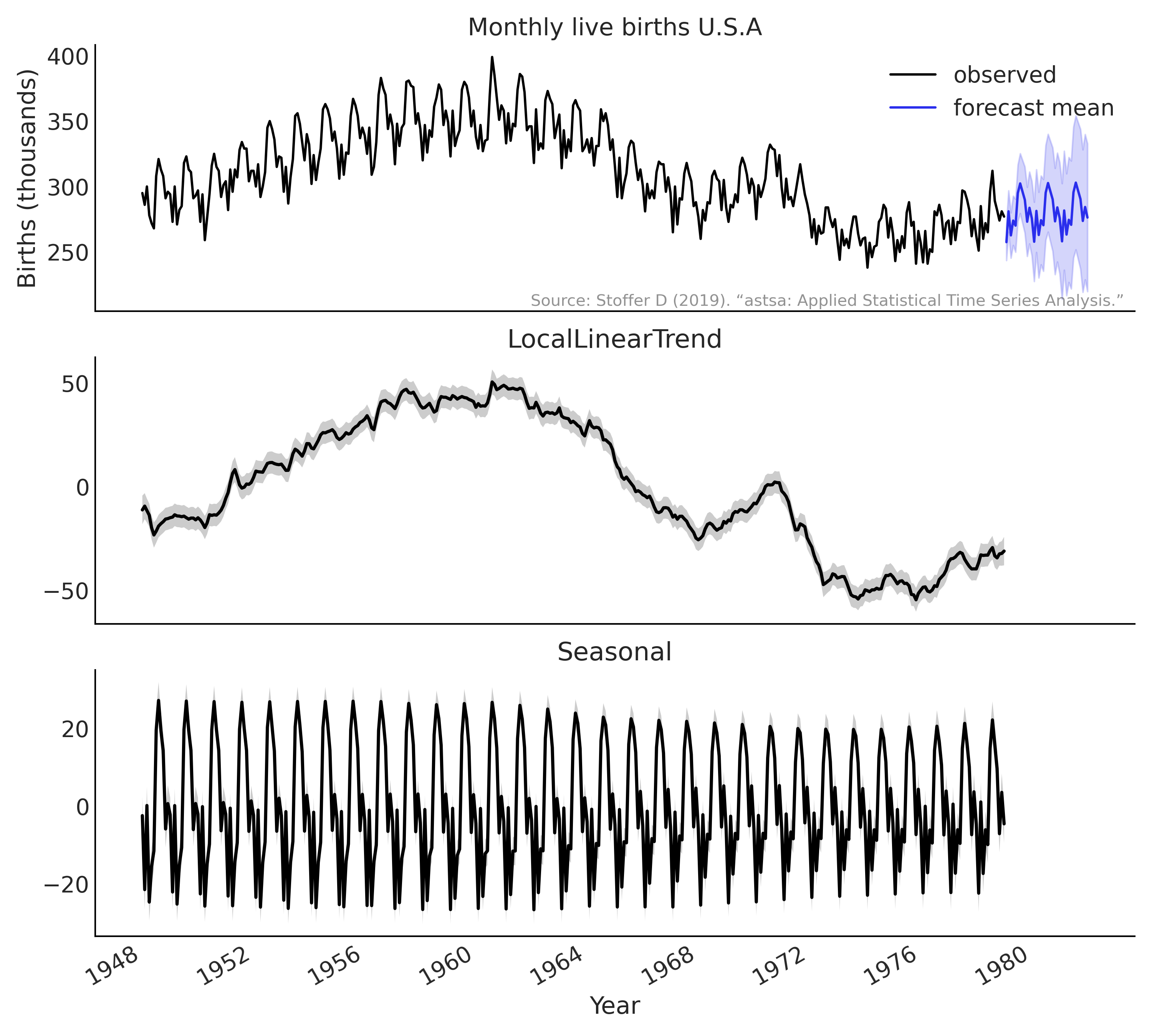
Fig. 118 使用带有代码 tfp_sts_example2_result 的 tfp.sts API 来推断美国（1948-1979 年）每月活产的结果和预测。顶图：\(36\) 个月的预测；下部的两个图：时间序列的结构化分解。

6.5 其他时间序列模型

虽然 结构化时间序列模型 和 线性高斯状态空间模型 强大且富有表现力，但它们无法满足我们的所有需求。因此有很多在其基础上的扩展，例如：

• 扩展卡尔曼滤波 ：可用于 非线性高斯状态空间模型 中 \(X_t\) 的推断。注：非线性指状态空间模型中的转移函数和观测函数是可微分的非线性函数。

• 无损卡尔曼滤波：可用于推断非高斯非线性模型 [62] 。

• 粒子滤波：可以作为状态空间模型的一般性滤波方法 [63] 。

• 隐马尔可夫模型：一种具有离散状态空间的状态空间模型。

另外，还存在一些模型推断的专用算法，例如：

• 前向后向算法：用于计算边缘后验似然。

• Viterbi 算法：用于计算后验的众数。

此外，还有作为连续时间模型的常微分方程 (ODE) 和随机微分方程 (SDE)。

在 Table 14 中，我们按照随机性和时间处理方式对模型进行了大致划分。它们都是经过深入研究的主题，在 Python 计算生态系统中具有易于使用的实现。

Table 14 按随机性和时间处理分类的各种时间序列模型

	Deterministic dynamics	Stochastic dynamics
Discrete time	automata / discretized ODEs	state space models
Continuous time	ODEs	SDEs

`

6.6 时间序列模型的评判和先验选择

在 Box et al. [57] 的开创性时间序列书中 15 ，概述了时间序列建模的五个重要实际问题：

• 预测

• 转移函数的估计

• 异常干预事件对系统的影响分析

• 多元时间序列分析

• 离散控制系统

大多数时间序列问题旨在执行某种预测（或即时预测，你试图在瞬时时间 \(t\) 推断一些由于获取测量滞后而尚不可用的观测量），这自然地建立了一个时间序列分析问题的模型评估标准。虽然我们在本章中没有围绕贝叶斯决策理论进行特定处理，但值得引用 West and Harrison [59] 的内容：

良好的建模需要认真思考，而良好的预测需要对预测在决策系统中的作用有一个综合认识。

6.6.1 时间序列模型的评估

（1） 绝对值百分比均值误差（MAPE）

在实践中，对 时间序列模型推断的评判 和 对预测的评估 应当与决策过程紧密结合，尤其是如何将不确定性纳入决策。虽然如此，我们还是能够单独对预测性能进行评估的。通常这种评估是通过收集新数据或留出一些测试数据来实现的，就像在本章对 \(\text{CO}_2\) 示例所做的那样，使用标准指标将观测结果与预测结果进行比较。其中有一种流行的选择是计算绝对值百分比均值误差 (MAPE)：

(69)\[MAPE = \frac{1}{n} \sum_{i=1}^{n} \frac{|\text{forecast}_i - \text{observed}_i|}{\text{observed}_i}\]

显然 MAPE 存在一些偏差，例如，在取值较低的观测中，一旦出现较大误差就会显著影响 MAPE 值。此外，当观测值范围差异较大时，难以跨多个时间序列进行 MAPE 比较。

基于交叉验证的模型评估方法仍然适用并推荐用于时间序列模型。但如果目标是评估对未来时间点的预测性能，则将 LOO 用于单个时间序列是有问题的。每次简单地留出一个观测值的方法没有考虑到数据（或模型）的时间结构。例如，如果你删除一个点 \(t\) 并将其余点用于预测而不考虑时间结构，那么你可以使用过去的点 \(t_{-1}, t_{-2}, ...\) 预测未来，但理论上你也可以使用未来的点 \(t_{+1}, t_{+2}, ...\) 来预测过去。因此，我们可以计算 LOO，但对其结果的解释将是荒谬的，会产生误导。

在时间序列模型的评估中，我们不需要留出一个（或一些）时间点，而是需要某种将未来数据留出的交叉验证形式（ Leave-Future-Out Cross-Validation, LFO-CV ），参见 Bürkner et al. [64]。其大概意思是，在初始模型推断之后，为了提前一步做出近似预测，可以在留出的时间序列上或未来观测数据上进行迭代，并基于对数预测密度做出量化评估；当某个时间点的帕雷托 \(k\) 估计值超出指定阈值时，将其纳入训练集重新拟合模型 16。 因此，LFO-CV 不是针对某个单一预测任务的交叉验证方法，而是面向未来时间点的各种可能预测任务的交叉验证方法。

6.6.2 时间序列模型的先验

在 6.2.3 基函数和广义可加模型 部分中，我们将正则化先验（拉普拉斯先验）用于阶跃线性函数的斜率，以表达我们的先验知识，即斜率变化通常很小且接近于零，因此产生的潜在趋势更为平滑。

（1）对假日事件的先验建模

正则化先验（或稀疏先验）还常用于对假日（或其他特殊日子）事件建模。通常每个假日都有自己的系数，如果我们想表达一个先验，即表明某些假日可能会对时间序列产生巨大影响，而其他大多数假日有普通日子一样，那么可以使用马蹄形先验 [65, 66] 将这种直觉形式化，如公式 (70) 所示：

(70)\[\begin{split}\begin{split} \lambda_t^2 \sim& \mathcal{H}\text{C}(1.) \\ \beta_t \sim& \mathcal{N}(0, \lambda_t^2 \tau^2) \end{split}\end{split}\]

马蹄形先验中的全局参数 \(\tau\) 将假日效应的系数全都拉向零。同时，局部尺度参数 \(\lambda_t\) 的重尾，使得在这种收缩中产生了一些暴发效应。我们可以调整 \(\tau\) 值来适应不同程度的稀疏性：\(\tau\) 越接近于零，假日效应 \(\beta_t\) 的收缩越趋向于零，而较大的 \(\tau\) 则对应一个更为分散的先验 [67] 17。例如，在 Riutort-Mayol et al. [68] 的案例研究 \(2\) 中，他们为一年中的每一天（包括闰日为 366 天）添加了一个特殊的日效应，并在对其进行正则化之前使用了马蹄形分布。

（2）对观测噪声的先验建模

时间序列模型先验的另一个重要考虑因素是观测噪声的先验。大多数时间序列数据本质上是非重复测量。我们根本无法及时返回并在确切条件下进行另一次观测（即，我们无法量化偶然不确定性）。这意味着我们的模型需要先验信息才能“确定”噪声是来自测量还是来自隐过程（即 epistemic 不确定性）。例如，在具有隐自回归分量或局部线性趋势模型的时间序列模型中，我们可以将更多信息先验放在观测噪声上，以将其调节为更小的值。这将“推动”趋势或自回归分量以过度拟合潜在的漂移模式，并且我们可能对趋势有更好的预测（短期内预测准确性更高）。风险在于我们对潜在趋势过于自信，从长远来看，这可能会导致预测不佳。在时间序列很可能是非平稳的实际应用程序中，我们应该准备好相应地调整先验。

习题

6E1. As we explained in Box Parsing timestamp to design matrix above, date information could be formatted into a design matrix for regression model to account for the periodic pattern in a time series. Try generating the following design matrix for the year 2021.

Hint: use Code Block timerange_2021 to generate all time stamps for 2021:

Listing 100 timerange_2021

datetime_index = pd.date_range(start="2021-01-01", end="2021-12-31", freq='D')

• A design matrix for day of the month effect.

• A design matrix for weekday vs weekend effect.

• Company G pay their employee on the 25th of every month, and if the 25th falls on a weekend, the payday is moved up to the Friday before. Try to create a design matrix to encode the pay day of 2021.

• A design matrix for the US Federal holiday effect 18 in 2021.

Create the design matrix so that each holiday has their individual coefficient.

6E2. In the previous exercise , the design matrix for holiday effect treat each holiday separately. What if we consider all holiday effects to be the same? What is the shape of the design matrix if we do so? Reason about how does it affects the fit of the regression time series model.

6E3. Fit a linear regression to the "monthly_mauna_loa_co2.csv" dataset:

• A plain regression with an intercept and slope, using linear time as predictor.

• A covariate adjusted regression like the square root predictor in the baby example in Chapter 4 Code Block babies_transformed.

Explain what these models are missing compared to Code Block regression_model_for_timeseries.

6E4. Explain in your own words the difference between regression, autoregressive and state space architectures. In which situation would each be particularly useful.

6M5. Does using basis function as design matrix actually have better condition number than sparse matrix? Compare the condition number of the following design matrix of the same rank using numpy.linalg.cond:

• Dummy coded design matrix seasonality_all from Code Block generate_design_matrix.

• Fourier basis function design matrix X_pred from Code Block gam.

• An array of the same shape as seasonality_all with values drawn from a Normal distribution.

• An array of the same shape as seasonality_all with values drawn from a Normal distribution and one of the column being identical to another.

6M6. The gen_fourier_basis function from Code Block fourier_basis_as_seasonality takes a time index t as the first input. There are a few different ways to represent the time index, for example, if we are observing some data monthly from 2019 January for 36 months, we can code the time index in 2 equivalent ways as shown below in Code Block exercise_chap4_e6:

Listing 101 exercise_chap4_e6

nmonths = 36
day0 = pd.Timestamp('2019-01-01')
time_index = pd.date_range(
    start=day0, end=day0 + np.timedelta64(nmonths, 'M'), 
    freq='M')

t0 = np.arange(len(time_index))
design_matrix0 = gen_fourier_basis(t0, p=12, n=6)
t1 = time_index.month - 1
design_matrix1 = gen_fourier_basis(t1, p=12, n=6)

np.testing.assert_array_almost_equal(design_matrix0, design_matrix1)

What if we are observing the data daily? How would you change the Code Block exercise_chap4_e6 to:

• Make time_index represent day of the year instead of month of the year.

• Modify the function signature to gen_fourier_basis in line 8 and 10 so that the resulting design matrices coded for the month of the year effect.

• How does the new design_matrix0 and design_matrix1 differ? How is the differences would impact the model fitting? Hint: validate your reasoning by multiplying them with the same random regression coefficient.

6E7. In Section 6.3 自回归模型 we introduced the backshift operator \(\mathbf{B}\). You might have already noticed that applying the operation \(\mathbf{B}\) on a time series is the same as performing a matrix multiplication. We can generate a matrix \(\mathbf{B}\) explicitly in Python. Modify Code Block ar1_without_forloop to use an explicit \(\mathbf{B}\) constructed in NumPy or TensorFlow.

6E8. The step linear function as defined in Equation (48) and Code Block step_linear_function_for_trend rely on a key regression coefficient \(\delta\). Rewrite the definition so that it has a similar form compare to other linear regression:

\[g(t) = \mathbf{A}^\prime \delta^\prime \]

Find the appropriate expression of design matrix \(\mathbf{A}^\prime\) and coefficient \(\delta^\prime\).

6E9. As we have seen in past chapters, a great way to understand your data generating process is to write it down. In this exercise we will generate synthetic data which will reinforce the mapping of “real world” ideas to code. Assume we start with a linear trend that is y = 2x, x = np.arange(90), and iid noise at each time point draw from a \(\mathcal{N}(0, 1)\). Assume that this time series starts on Sunday June 6 2021. Generate 4 synthetic datasets that include:

1. An additive weekend effect where weekends have 2x more volume than weekdays.

2. An additive sinusoidal effect of sin(2x).

3. An additive AR(1) latent process with autoregressive coefficient of your choice and a noise scale \(\sigma = 0.2\).

4. A time series with weekend and sinusoidal effect from (1) and (2), and an AR(1) process on the mean of the time series with the same autoregressive coefficient as in (3)

6E10. Adapt the model in Code Block gam_with_ar_likelihood to model the generated time series in 6E9 (4).

6E11. Inspection of the inference result (MCMC trace and diagnostic) of models in this chapter using ArviZ. For example, look at:

• Trace plot

• Rank plot

• Summary of posterior sample

Which model contains problematic chains (divergence, low ESS, large \(\hat R\))? Could you find ways to improve the inference for those models?

6M12. Generate a sinusoidal time series with 200 time points in Python, and fit it with a AR(2) model. Do that in TFP by modifying Code Block ar1_without_forloop and in PyMC3 with pm.AR API.

6M13. This is an exercise of posterior predictive check for AR models. Generate the prediction distribution at each time step \(t\) for the AR2 model in Exercise 6M11. Note that for each time step \(t\) you need to condition on all the observations up to time step \(t-1\). Does the one-step-ahead predictive distribution match the observed time series?

6M14. Make forecast for 50 time steps using the AR2 models from Exercise 6M11. Does the forecast also look like a sinusoidal signal?

6H15. Implement the generative process for the \(\text{SARIMA}(1, 1, 1)(1, 1, 1)_{12}\) model, and make forecast.

6M16. Implement and inference a \(ARIMAX(1,1,1)X[4]\) model for the monthly birth dataset in this chapter, with the design matrix generated from a Fourier basis functions with \(N=2\).

6H17. Derive the Kalman filter equations. Hint: first work out the joint distribution of \(X_t\) and \(X_{t-1}\), and then follow with the joint distribution of \(Y_t\) and \(X_t\). If you are still stuck take at look at Chapter 4 in Särkkä’s book [60].

6M18. Inspect the output of linear_growth_model.forward_filter by indexing to a given time step:

• Identify the input and output of one Kalman filter step;

• Compute one step of the Kalman filter predict and update step using the input;

• Assert that your computation is the same as the indexed output.

6M19. Study the documentation and implementation of tfp.sts.Seasonal, and answer the following questions:

• How many hyperparameters does a seasonal SSM contains?

• How does it parameterized the latent states and what kind of regularization effect does the prior has? Hint: draw connection to the Gaussian Random Walk prior in Chapter 5.

6M20. Study the documentation and implementation of tfp.sts.LinearRegression and tfp.sts.Seasonal, and reason about the differences of SSM they represent when modeling a day of the week pattern:

• How is the day of the week coefficient represented? Are they part of the latent states?

• How is the model fit different between the two SSMs? Validate your reasoning with simulations.

参考文献

https://github.com/asael697/bayesforecast.

---

1

https://quoteinvestigator.com/2013/10/20/no-predict/

2

There is also a subtlety that not all periodic patterns in the time series should be considered seasonal. A useful distinction to make is between cyclic and seasonal behavior. You can find a nice summary in https://robjhyndman.com/hyndsight/cyclicts/.

3

This makes the observation not iid and not exchangeable. You can also see in Chapter 4 where we define residuals

4

Which, it is unfortunate for our model and for our planet.

5

A series is stationary if its characteristic properties such as means and covariances remain invariant across time.

6

https://facebook.github.io/prophet/.

7

A demo of the design matrix used in Facebook Prophet could be found in http://prophet.mbrouns.com from a PyMCon 2020 presentation.

8

That is why is called autoregressive, it applies a linear regression to itself. Hence the similar naming to the autocorrelation diagnostic introduced in Section 2.4.5 自相关图.

9

Actually, the AR example in this section is a Gaussian Process.

10

The Stan implementation of SARIMA can be found in e.g.

11

For brevity, we omitted the MCMC sampling code here. You can find the details in the accompanying Jupyter Notebook.

12

It might be useful to first consider “space” here being some multi-dimensional Euclidean spaces, so \(X_t\) and \(Y_t\) is some multi-dimensional array/tensor when we do computations in Python.

13

This also gives a nice example of a non-stationary observation matrix \(\mathbf{H}\).

14

Note that this is not the only way to express ARMA model in a state-space form, for more detail see lecture note http://www-stat.wharton.upenn.edu/~stine/stat910/lectures/14_state_space.pdf.

15

Nothing more puts George E. P. Box’s famous quote: “All models are wrong, but some are useful” into perspective, than reading through his seminal book and working on forecasting problems.

16

For a demonstration see https://mc-stan.org/loo/articles/loo2-lfo.html.

17

Note that in practice we usually parameterize Equation (70) a little bit differently.

18

https://en.wikipedia.org/wiki/Federal_holidays_in_the_United_States#List_of_federal_holidays

previous

第五章: 样条

next

第七章：贝叶斯加性回归树